Kirja
| Site: | MyCourses |
| Course: | CHEM-E4175 - Fundamental Electrochemistry, 09.01.2019-18.02.2019 |
| Book: | Kirja |
| Printed by: | Guest user |
| Date: | Saturday, 13 July 2024, 8:31 PM |
Description
Table of contents
- 1. Electrochemical system
- 2. Thermodynamics of electrolyte solutions
- 3. Transport in electrolyte solutions
- 4. Electrochemical cells
- 5. Electrical double layer and adsorption
- 6. Electrochemical reaction kinetics
- 7. Electrochemical methods
- 8. Impedance technique
- 8.1. Basic elements of impedance
- 8.2. Graphical representations of impedance
- 8.3. Determining the impedance of an electrochemical system
- 8.4. Adsorption
- 8.5. Other diffusion elements
- 8.6. Corrosion
- 8.7. Dispersion of time constants
- 8.8. Transmission lines
- 8.9. Kramers-Kronig transforms
- 8.10. Similarities of the equivalent circuits
- 8.11. Some remarks on the experimental arrangement of impedance measurements
- 9. Electrochemical energy conversion
- 10. List of symbols
- 11. Appendices
1. Electrochemical system
1.1. What is electrochemistry?
Electrochemistry studies the physical properties of electrically charged particles and their systems as well as their reactions and transport in the system. An electrochemical system thus consists of charged particles and a medium, i.e. a solvent, most commonly water. Particles and the medium form an electrolyte solution. Particles are usually ions, ion complexes or macromolecules, but also a free solvated electron can exist in a solution. Solid electrolytes and molten salts are special cases of electrolyte solutions; they require very high operation temperatures, typically approximately 800 ºC. The former are used in solid oxide fuel cells and the latter in the production of, for example, aluminum. Recently, ionic liquids aka room temperature molten salts have received a lot of attention. They are salts assembled from large organic molecules that can be liquid at room temperature or at slightly elevated temperatures (less than 100 °C).
An electrochemical system also contains electrodes. They are needed because an electrochemical reaction is always heterogeneous, taking place on a solid surface containing free electrons or at some other interface between the electrolyte solution and a phase containing charged species. Electrodes are typically metals or other solids with good electrical conductivity, such as graphite. In order to understand the nature of an electrode reaction, the electron structure of solid materials is briefly addressed in the end of this chapter. Electrodes are connected to each other via an external electrical circuit that can be as simple as a copper wire, but most commonly a load (a resistor) and/or a measurement instrument. An ensemble formed of an electrolyte solution, electrodes and an external circuit is called as an electrochemical cell.
Thermodynamics is a discipline with which the properties of electrolyte solutions can be studied. Due to long-range electrical (coulombic) interactions, the properties of electrolyte solutions are very different from solutions of electrically neutral solutes; this is addressed in detail in Chapter 2. Electrode reactions create local concentration differences in an electrolyte solution that transport processes try to level out. The analysis of transport processes therefore constitutes an essential part of the study of an electrochemical system. Transport is addressed in Chapter 3.
Yet another special feature of electrochemical reactions is that in addition to temperature, pressure and concentration, their rate depends, like most reactions, on the potential of the electrode. Potential has several bearings in electrochemistry as addressed in the end of this chapter. Since reaction rates depend on potential in an exponential manner as explained in Chapter 6, reaction rates can be controlled over several orders of magnitude.
1.2. Electrochemical reaction
An electrochemical reaction involves always electron transfer between species. Such a reaction is called a redox reaction. It is defined:
Oxidation means donating an electron and reduction accepting an electron. |
|---|
A substance capable of oxidizing another substance is knows as an oxidant. Accordingly, a reducing
substance is a reductant. If we
write down a reaction
| Aox + Bred → Ared + Box , | (1.1) |
|---|
where n electrons are transferred from B to A, A is the oxidant of B and B is the reductant of A. Hereinafter in this book, the subscripts ’ox’ and ’red’ refer to the oxidized and reduced species, respectively.
The ability of a substance to oxidize or reduce another substance depends on their electron structure and, to a lesser extent, on the medium. This ability is reflected in the values of the standard reduction potentials that are tabulated for several elements and molecules. Standard potentials are discussed in Chapter 4, and a selection of the most common redox couples is given in Appendix 6. From the standard potentials it is possible to deduce which reactions would occur spontaneously or how much energy must be fed in to the system to force a reaction to take place.*
If an electron transfers from a species in the solution to another species without a mediating electrode, electron transfer is homogeneous. For example, if an aqueous solution of CeCl4 and FeCl2 are shaken for a while, Ce4+ oxidizes Fe2+ to Fe3+ reducing to Ce3+. In biology, redox reactions are mostly homogeneous. Metals can also be reduced from aqueous solutions with strong reductants without an external circuit. One of the best known processes is the deposition of nickel from a hypophosphate solution. This kind of processes are known as electroless plating. They do not, however, represent true homogeneous electron transfer because a solid surface mediates electrons and other simultaneous reactions compensate the transferred charges.
A redox reaction is electrochemical if electron transfer takes place heterogeneously, most commonly on solid electrodes.
Electrochemical reaction is a heterogeneous redox reaction. |
|---|
An alternative definition would be
Rate of an electrochemical reaction depends on potential. |
|---|
Electrodes traditionally used in electrochemistry are made of solid materials that have sufficient electrical conductivity, such as metals, graphite or indium-titan oxide glass (ITO). An electrode exchanges an electron with a reacting species, and receives an electron from an external circuit or donates an electron to it. The surface of an electrode can be modified with functional groups in order to enhance its selectivity towards a particular reacting species.
As a result of a redox reaction, an imbalance of charges is created in the solution, and another electrode must be inserted in the system to maintain electroneutrality in the solution. The electrodes must be connected via an external circuit. Reaction (1.1) can now be written in terms of electrode reactions as follows:
| Aox + ne– → Ared reduction
at the cathode |
(1.2a) |
|---|---|
| Bred → Box+ ne– oxidation at the anode | (1.2b) |
Summing reactions (1.2a) and (1.2b) gives reaction (1.1). In reaction (1.2a) the electrode donates n electrons to Aox: it is a cathode. In reaction (1.2b) the other electrode receives the same number of electrons: it is an anode.
Reactions (1.2) and (1.2b) are the half-reactions of reaction (1.1). If we want to study, say, the rate of the half-reaction (1.2a), the cathode is called the working electrode, and the anode that only balances the number of charges in the solution the counter electrode or the reference electrode. In modern electrochemical measurement, the counter and reference electrodes are separate – this will be discussed in Chapter 4.7.
Electron transfer is a fundamental reaction which is very difficult to describe with quantum mechanics. Theories of electron transfer have traditionally been based on the famous Arrhenius equation or the absolute rate theory (aka theory of activated complexes) by Eyring. The rate of electron transfer, in other words electric current, is, however, easily measured and controlled in situ, making electrolysis a widely used chemical process.
1.2.1 Cell voltage due to an electrochemical reaction
Let’s write down a very simple and familiar reaction:
| H2(g) + ½ O2(g) → H2O(l) | (1.3) |
|---|
It is found from thermodynamic tables that the standard Gibbs free energy of the reaction is \( \Delta \)G0 = –237 kJ mol–1. The reaction does not appear electrochemical but it is the net reaction of the hydrogen fuel cell in acidic conditions. At the anode of the fuel cell, hydrogen decomposes by means of a catalyst (oxidizes):
| H2 → 2 H+ + 2 e– | (1.4) |
|---|
Protons are transported to the cathode through the electrolyte and electrons via the external circuit. At the cathode, oxygen is reduced:
| ½ O2 + 2 H+ + 2 e– → H2O | (1.5) |
|---|
The sum of reactions (1.4) and (1.5) is reaction (1.3). What does this mean? The homogeneous reaction (1.3) has been split into two heterogeneous electrode reactions. The cell voltage is defined as follows:
\( \displaystyle E=-\frac{\Delta G}{nF} \) |
(1.6) |
|---|
Two electrons are transported per water molecule. Hence, the standard cell voltage (or potential) is
\( \displaystyle E^0=\frac{237000\text{ J/mol}}{2 \cdot 96485 \text{ As/mol} } \)
the thermodynamic (= equilibrium) potential of the hydrogen fuel cell**.
Thus, in electrochemistry, a homogeneous reaction is split into two heterogeneous reactions and the Gibbs free energy of the reaction, \( \Delta \)G, is harnessed as electrical energy. In a reverse process, electrical energy can be used to run reactions against their natural affinity. The question of how \( \Delta \)G of the total reaction is split between the half-reactions remains still unanswered. As will be seen in Chapter 4, thermodynamics is incapable of answering this question, but it is resolved with an IUPAC resolution. This does not actually matter because measuring a single electrode potential, i.e. its energy, is not possible, only the potential difference between two electrodes can be measured.
1.2.2 Electric current due to an electrochemical reaction
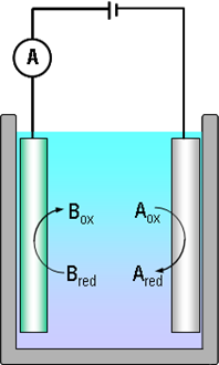
Consider electric current with the help of reactions (1.2) and Figure 1.1. The electrons that Bred donates to the anode are transported to the cathode via the external circuit, making the measurement of current feasible. Because the rate at which Bred donates the electrons is equal to the rate at which Aox receives them and that is equal to the electron flux in the external circuit, electric current is proportional to the reaction rate. This fundamental notion is known as Faraday's law:\( i=nFr \) |
(1.7) |
|---|
where i is electric current density (A cm–2), n the number of electrons exchanged in the reaction, F the Faraday constant (96485 As mol–1) and r the reaction rate (mol cm–2 s–1). The direction of electric current is defined as the direction of positive current, i.e. opposite to the direction of electrons. In a solution, the current flows in the direction of the positively charged species. When representing current-voltage curves in x-y coordinates, it is still necessary to agree if an oxidation or reduction current is positive: according to the IUPAC resolution, an oxidation current is positive. Many text books, however, especially ones about polarography, show cathodic current (reduction current) as positive. Great care must therefore be taken when reading literature and noticing the sign convention used by authors.
It is necessary to emphasize that an electrochemical reaction is the only reaction, the rate of which can be measured in situ. With modern current amplifiers, the measurement of pA (10–12 A) currents is rather easy. Applying the Faraday law it is simple to calculate that this corresponds to the transfer of the order of 106 electrons per second.
Since electric current is a property of a closed circuit, its magnitude depends on the rate of the slower reaction. Let’s assume that the reduction reaction (1.2a) is faster than the oxidation reaction (1.2b). If the electrodes in Fig. 1.1 are short-circuited, electric current density is i = nFrox because the rate of the oxidation reaction limits the rate of electron flow. Superficially thinking, this observation may seem self-evident but it has a huge impact in the production of metals via electrolysis where oxygen evolution is the anode reaction. The rate of oxygen evolution (inverse of reaction (1.5)) is limited by reaction kinetics, increasing the cell voltage by several hundred millivolts which, in turn, increases the energy cost of the process significantly.
* Standard potentials are thermodynamic quantities, but sometimes reaction kinetics determines which reaction prevails in the system. The electrolysis of zinc is a famous example of the kinetic control.
**Note that J = VAs
1.3. Properties of electrodes
1.3.1 Electron structure of solid materials
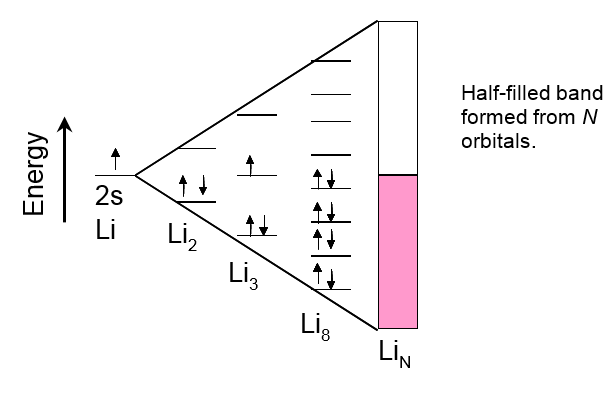
Electrodes are typically solid, metallic materials. In order to understand reactions taking place on them, it is useful to examine the structure of solid metals. A simple approach is to consider the structure as an ensemble of tightly packed lattices of atomic nuclei and electrons that are partly moving freely within the lattice. Let us concentrate on the cloud of these free electrons and study its emergence with an example. Lithium is the lightest alkali metal, its electron configuration is 1s22s1. It has one electron more than a noble gas (e.g. He). Two lithium atoms form a molecule Li2. The molecular orbital theory tells that from the two atomic 2s orbitals of lithium, two molecular orbitals are formed in a Li2 molecule: a binding orbital \( \sigma \)2s that resides between the Li nuclei, and an anti-bonding orbital \( \sigma \)*2 s on the opposite sides of the nuclei. According to the Aufbau principle, the 2s electrons of the lithium atoms that participate in the bond formation are filling the binding molecular orbital; the four 1s electrons stay on their atomic orbitals. Bringing more Li atoms into the system means more molecular orbitals are formed, including anti-bonding orbitals. Upon this process, the energy levels of the bonding orbitals get closer to each other, ultimately forming a continuous energy band when the number of atoms becomes high (molecule LiN), see Figure 1.2. Binding electrons, one electron for each Li atom, occupy only half of this band known as the valence band.
In terms of energy, below the valence band there is a band of 1s electrons that is fully occupied (not shown in Figure 1.2). Between this band and the valence band, there is an energy gap that is so wide that no 1s electron can rise to the valence band. Above the valence band there is a conduction band that is unoccupied at ground state. (Figures 1.2 and 1.3). In the case of lithium, it is formed from the molecular orbitals that are left unoccupied. Their energy is higher than that of the occupied orbitals by such small an amount that thermal energy (kBT) is capable of raising electrons to them, making lithium electronically conducting. Metals, in general, are good electronic conductors because their valence electrons are delocalized within the entire lattice.
Considering alkaline earth metals such as
magnesium in the similar manner, the situation changes somewhat. Molecular
orbitals formed from atomic 3s orbitals would be fully occupied by the 3s
electrons of Mg. So why are alkaline earth metals also good electronic conductors? Let us continue with the example
of Mg. Molecular orbitals are also formed from the atomic orbitals that are unoccupied at ground state (3p orbitals). Again, when the number of atoms is
high, the energy levels of these unoccupied molecular orbitals form a continuous
band. In magnesium, this band partly overlaps with the valence band, making the
exchange of electrons between the valence and conduction band feasible, see Figure
1.3.
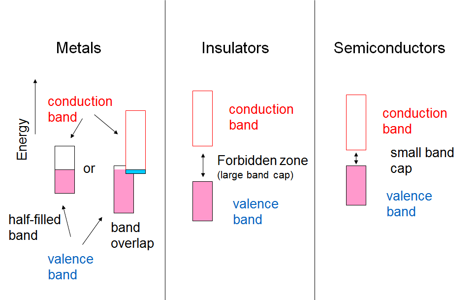
Electrical conductivity can be reduced to the issue of the band gap between the valence and conduction bands, as shown in Figure 1.3. If the band gap is of the order of 5 eV or higher, the material is an insulator because thermal energy (kBT = 0.025 eV at 300 K) is not capable of raising an electron from the valence band to the conduction band. If the band gap is of the order of 1-2 eV, some electrons can be raised to the conduction band, and the material is a semi-conductor. The conductivity of semi-conductors increases with temperature, in other words thermal energy, while the conductivity of metals decreases because the thermal motion of the metal nuclei interferes the free transfer of electrons. This is used as the definition of a metal.
1.3.2 Fermi levels and work function in solids
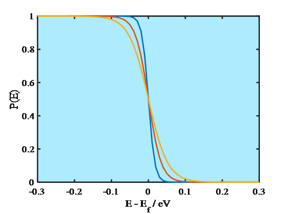
Electrons are fermions obeying the Pauli exclusion principle that two electrons cannot have the same quantum state in a system. As the consequence, electrons do not occupy the energy levels according to the Boltzmann but the Fermi-Dirac distribution. The probability P of finding an electron on an energy level E is
| \( \displaystyle P(E)=\frac{1}{1+e^{(E-E_f)/kT}} \) | (1.8) |
|---|
where Ef is the Fermi energy. At absolute zero (0 K) the energy levels are occupied according to the Aufbau principle, starting from the lowest energy level. The energy of the highest occupied molecular orbital, HOMO, is known as the Fermi energy that is also equal to the electrochemical potential of an electron. As Equation (1.8) manifests, at 0 K the probability of finding an electron on an energy level E < Ef is unity and on a level E > Ef zero. Since the electrochemical potential of an electron in a metal does not change significantly as a function of temperature, it has been common to call the energy where the step function occurs the Fermi level. At higher temperatures, however, Fermi-Dirac distribution is no longer a step function but changes smoothly, as shown in Figure 1.4. Yet, the distribution takes values different from unity or zero only around the energy where P(E) = 0.5, which is the definition of the Fermi level. The Fermi level is sometimes defined as the lowest energy of the conduction band of a solid which makes it possible to give numerical values to the Fermi level with respect to a reference point.
In solid state physics, metals are often sorted according to their work function, \( \Phi \), which is the work (energy) required to remove an electron from an uncharged metal, that is, from its Fermi level. The work function can be measured via, for example, the photoelectric effect. The work function is in practice a temperature-independent quantity, but it is important to note that it does depend on the lattice structure of a material. Work functions of metals vary from 2.3 eV of potassium to 5.3 eV of gold.
1.3.3 Potential and voltage
Potential is one of the most versatile and salient quantities in electrochemistry. Voltage is often used as a synonym for potential, but voltage is a measurable quantity while only potential differences can (possibly) be measured. Voltage can thus be defined as the potential difference between two points that can be a sum of several contributions. The free energy of the net electrochemical reaction is converted to the cell voltage according to Equation (1.6) which is the sum of the contributions of the anode and cathode reactions. Free energy is the driving force of a reaction and a measure of its tendency to take place, and we know from thermodynamics that spontaneous reactions have negative Gibbs free energies. Therefore, from Equation (1.6), positive cell voltages mean spontaneous reactions that produce energy, for example in a battery.
Although thermodynamics is not capable of resolving the free energy of individual electrode reactions, but an assumption is made to fix the potential scale (Chapter 4), we can elaborate the potential of a solid electrode a little bit further. The potential of a solid electrode – be it metal or semiconductor – can be considered a measure of the Fermi level of electrons in the electrode. From electrostatics we know that an extra electric charge creates potential. If an electrode carries a net negative charge its potential is negative with respect to an uncharged electrode or to an electroneutral solution. A positive charge obviously means positive potential. With electrochemical instrumentation, we can control the electrode potential externally which means controlling the Fermi levels or, alternatively, the charge of an electrode.
Let us consider further potential related quantities encountered in electrochemistry. The inner phase of any material is electroneutral. If an object carries an electric charge it is spread over its surface. The potential measured on the surface of an object or in its immediate proximity, with respect to vacuum, is the outer potential, \( \ \psi \). This is the work required to bring an elementary charge from an infinite distance in a vacuum to the surface of a phase (see Figure 1.5). The outer potential can be measured using a Kelvin probe. It follows from the previous paragraph that a negatively charged object has a negative outer potential and a positively charged one a positive outer potential. The potential difference between two charged objects is also known as the Volta potential difference.
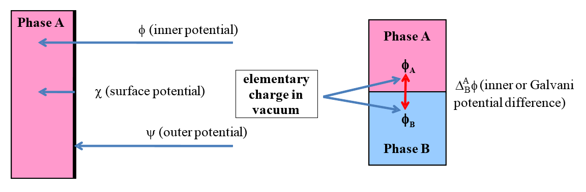
Figure 1.5. Left: Definitions of the inner or Galvani potential (\( \phi \)), surface potential (\( \ \chi \)) and outer potential (\( \psi \)). Right: Galvani potential difference between two phases.
\( \chi \) is the surface potential, the work required to bring an elementary charge from the surface of an object into its interior. The surface potential cannot be measured. The origin of the surface potential is the difference in the molecular (or atomic) interactions on the surface and in the interior of a material. In solids and liquids, molecules (atoms) residing on the surface experience asymmetric attraction towards the interior that gives them higher energy than that of the bulk of the material. Inserting a charged electrode into a polar solvent, the solvent molecules are oriented in a particular manner, creating surface dipoles. Now surface potential is created across the layer of these dipoles. The inner or Galvani potential, \( \phi \), is the total work required to bring an elementary charge from a vacuum to the inside of a phase. Based on what is stated above (and Figure 1.5), the Galvani potential can be expressed as the sum of the outer and surface potentials:
| \( \phi=\psi+\chi \) | (1.9) |
|---|
Galvani potential cannot be measured. On the right of Figure 1.5, the Galvani potential difference is defined. That can be measured under certain experimental arrangements (Chapter 4). Because the interiors of the both phases are electroneutral, Galvani potentials are constant within the materials and the Galvani potential difference is always formed at the interface between the phases.
1.3.4 Electron transfer on an electrode
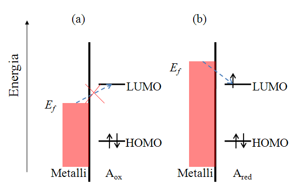
Let us consider the reduction reaction (1.2a) in a qualitative manner. Species A has an electronic structure based on the molecular orbital theory, as depicted in Figure 1.6. In order to reduce A, an electron must be transferred to its lowest unoccupied molecular orbital (LUMO). In Figure 1.6a, the Fermi level of the electrode is not sufficiently high to inject an electron to A, but as the electrode potential is changed so that the Fermi level is set higher than that of the LUMO of A (Figure 1.6b), and electron transfer becomes feasible. It is necessary to emphasize that an electron in the solution, or merely in the solute dissolved in the solvent, has no unambiguously defined energy. It is commonly assumed that its energy demonstrates Gaussian distribution and depends on the solvent-solute interactions. The Fermi level of an electron in the solution is defined as its electrochemical potential (see Chapter 6).
The rates of electron transfer can vary in the range of several orders of magnitude. This property can be quantified as the polarizability of an electrode. Polarizability is simply a measure of the dependence of the electron transfer rate on the electrode potential. An ideally non-polarizable electrode does not change its potential when current is flowing through it, while the potential of an ideally polarizable electrode can be varied without current flowing, see Figure 1.7.
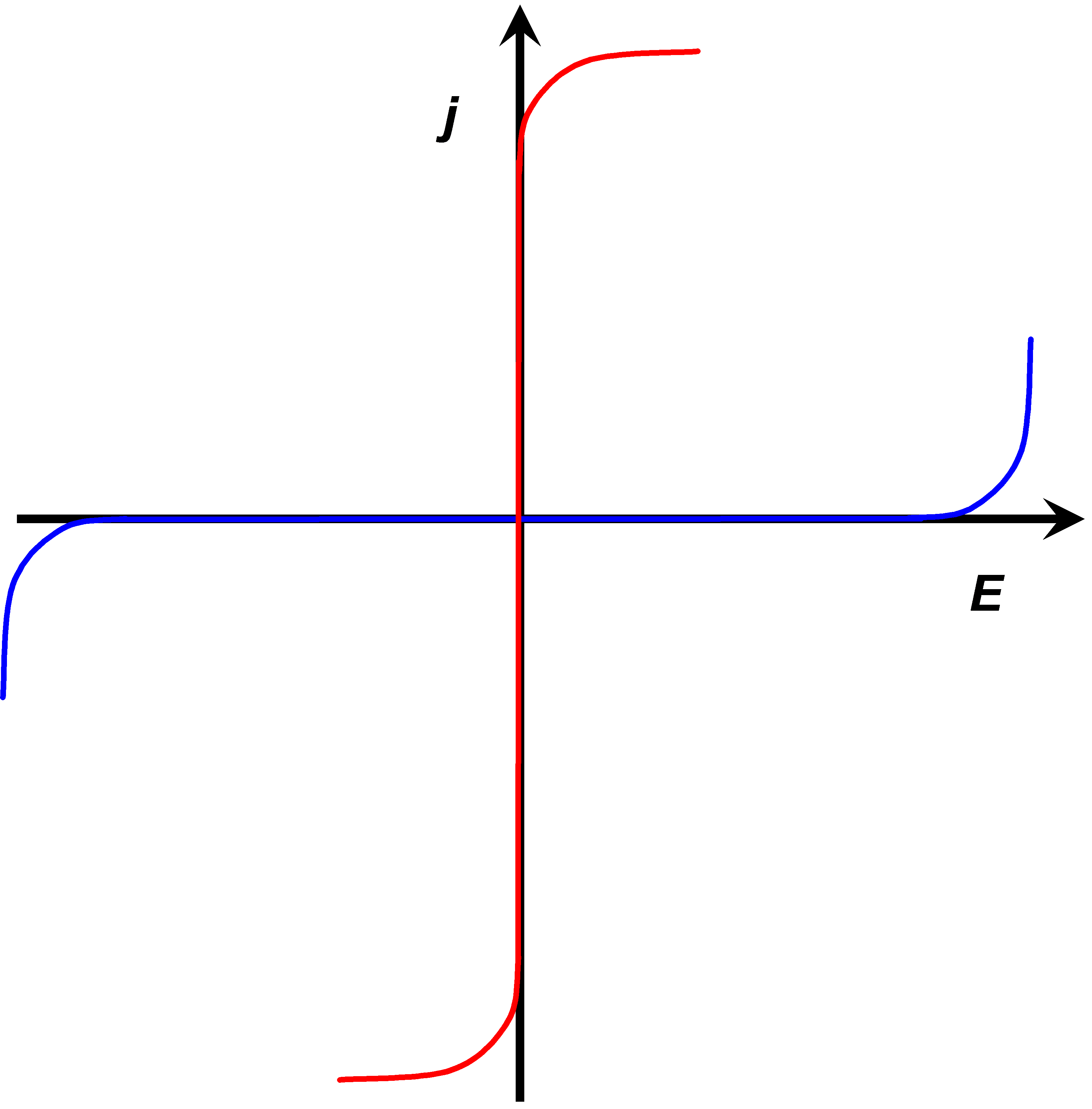
The rate of electron transfer in an ideally non-polarizable electrode is infinitely high, while the rate in an ideally polarizable electrode is zero. Ideal electrodes do not naturally exist but a Ag/AgCl electrode is non-polarizable to a significant extent. Its exchange current density (see paragraph 6.2.2) can be as high as 10 A cm–2. Perhaps the best polarizable electrode is the mercury drop. Its potential can be varied in the range of ca. 2.5 V without electrode reactions. The range of this potential window is determined by water splitting that is kinetically hindered on mercury. The electrode surface can also be modified in order to make it polarizable. Grafting an inert chemical group onto the surface, such as the diazonium moiety on graphite, the potential window can be extended to almost 4 V.
You can now test your conceptual knowledge by taking Quiz Chapter 1.
2. Thermodynamics of electrolyte solutions
An electrochemical system consists of electrodes and an electrolyte solution. The essential feature of an electrolyte solution is that it contains free species that carry electric charge. Charged species interact with their environment with long-range coulombic forces which make the properties of an electrolyte solution very different from those of a solution of electrically neutral species. In this chapter, we discuss the fundamentals of the thermodynamics of electrolyte solutions. More advanced and detailed treatises are given by Bockris and Reddy [1] or Harned and Owen [2].
[1] J.O’M. Bockris, A.K.N. Reddy, Modern Electrochemistry, vol 1, 2. p. Plenum Press, New York 1988.
[2] H.S. Harned, B.B. Owen, Physical Chemistry of Electrolyte Solutions, Reinhold Publishing Company, New York 1943.
2.1. Species and components
All the entities existing in a system – ions, molecules, electrons etc. – are called species, while components are those species the amount of which can be varied independently. For example, an aqueous solution of acetic acid contains the species H+, OH–, H2O, CH3COO– and CH3COOH, but only two components, H2O and CH3COOH. A proton (or more like H3O+) and a hydroxyl ion OH– are coupled with the ionic product of water:
\( K^w = {[\text{H}^+]} [\text{OH}^-] =10^{-14} \) at 25 °C | (2.1) |
|---|
The dissociation constant of acetic acid couples H+, CH3COO– and CH3COOH:
\(\ce{ ${K}_\ce{a}$=$\frac{[\ce{H+}][\ce{CH3COO-}]}{[\ce{CH3COOH}]}$ }\)\( =1.7378 \times10^{-5} \text{M} \) at 25 °C | (2.2) |
|---|
Furthermore, electrolyte solutions obey the very strong condition of (local) electroneutrality:
\( \displaystyle\sum\limits_{i}z_ic_i=0 \) | (2.3) |
|---|
The general statement
is that if a system contains N species, bound by m reactions and p
other contraints, the number of components, M,
is
M = N - m - p | (2.4) |
|---|
In acetic acid, N
= 5, m = 2 and p = 1, hence M = 2. Equation (2.4) can be
generalized to the Gibbs phase rule.
Assume that acetic acid is distributed between an aqueous and an organic
solvent phase (o). In addition to the above mentioned aqueous species, the
entire system contains (at least in principle) the species H+(o), OH-(o),
CH3COO-(o),
CH3COOH(o) and the
organic solvent, making N equal to 10. The mutual solubility of water
and the organic solvent is assumed to be negligible. Yet an extra variable is
the Galvani potential difference created across the phase boundary. The
constraints are two reactions, the
electroneutrality condition and four partition equilibria. The Galvani
potential difference can be eliminated with the total mass balance of acetic
acid. M thus is three, the components being water, acetic acid and the
organic solvent. Electroneutrality in water implicitly implies electroneutrality in the organic phase too. Writing ionic equilibria similarly to (2.1) and (2.2)
in the organic phase does not result in extra constraints either. Furthermore, it
should be noted that the Gibbs-Duhem equation
\( \displaystyle\sum\limits_{i} \mu _idn_i=0, \) p, T constants | (2.5) |
|---|
gives an extra constraint that in the both phases there is only one thermodynamically independent component, the solvent or acetic acid, hence two totally independent components.
2.2. Chemical potential
We already introduced the chemical potential \( \mu_i \) of component i in the Gibbs-Duhem equation. It is defined as
\( \displaystyle\mu_i= \left( \frac{\partial G}{\partial n_i} \right) _{P,T,n_{j \neq i }}=\mu_i^0+RT\ln a_i \), | (2.6) |
|---|
where G is the Gibbs free
energy of the solution. For ions, an electrochemical potential can be defined as
\( \displaystyle\tilde{\mu_i}= \mu_i+z_iF \phi= \mu_i^0+RT\ln a_i+z_iF \phi \) | (2.7) |
|---|
where F is the Faraday constant, zi the charge number, \( \mu_i^0 \) is the standard chemical potential and ai is the activity of ion i, respectively. Thus, for an uncharged species \( \tilde{\mu_i}=\mu_i \). Definition (2.6) is not, however, relevant for an ion because it is not possible to change the concentration of a single ion while keeping the concentrations of the other ions constant.
The fundamental Gibbs
equation expresses the change of the system’s internal energy dU as
dU = dq + dw = TdS - PdV only PV work | (2.8) |
|---|
where q is heat evolved from the system or exchanged with its environment, and dw is the work done against the system. In addition to the PV work it can contain, for example work against surface tension, \( \gamma dA \), or electrical work, \( \phi \)dqe. (\( \gamma \) is surface tension, qe electric charge and \( \phi \) electric potential.)
The other thermodynamic state functions, H (enthalpy), F (Helmholzin free energy) and G are easily derived from Equation (2.8):
\( H=U+PV \Rightarrow dH=dU+PdV+VdP=TdS+VdP \) | (2.9) |
|---|
\( F=U-TS \Rightarrow dF=dU-TdS-SdT=-SdT-PdV \) | (2.10) |
|---|
\( G=H-TS \Rightarrow dG=dH-TdS-SdT=-SdT+VdP \) | (2.11) |
|---|
In all these functions, the term \( \sum\limits_{i}\mu_idn_i \) can be added that takes into account the amount of material in the system. Adding the term that takes into account ions,\( \sum\limits_{i}\tilde{\mu_i}dn_i \), into Equation (2.11) gives
\( dG=-SdT+VdP+\sum\limits_{i}(\mu_i+z_iF\phi)dn_i \) \( =-SdT+VdP+\sum\limits_{i}\mu_idn+F\phi\sum\limits_{i}z_idn_i \) \( =-SdT+VdP+\sum\limits_{i}\mu_idn_i+F\phi dq_e\) | (2.12) |
|---|
where the definition of the electric charge \( q_e=\sum\limits_{i}z_in_i \) is used. In an electroneutral system \( q_e=0 \), but as will be seen later on, the concept of the electrochemical potential is most useful. The Galvani potential \( \phi \) also is conceptually a bit problematic; in metals it is related to the Fermi energy of electrons (see paragraph 1.3.3). Anyway, applying the equality of the electrochemical potential between the phases at equilibrium, Galvani potential differences between phases and the electromotive force (Chapter 4) can be derived. In the Gibbs-Duhem Equation (2.5) the chemical potential can thus be replaced by the electrochemical potential.
2.3. Activity
2.3.1 Activity of non-electrolytes
In the expression of the chemical potential (2.6), activity ai is introduced. It describes the ‘effective’ concentration of a solute, i.e. its deviation from ideal behavior. Depending on the concentration scale, the chemical potential can be written in different ways:
\( \mu_i=\mu_i^{0,x}+RT\ln(f_ix_i) \) mole fraction scale | (2.13a) |
|---|
\( \mu_i=\mu_i^{0,m}+RT\ln(y_im_i) \) molality scale | (2.13b) |
|---|
\( \mu_i=\mu_i^{0,c}+RT\ln( \gamma _ic_i) \) molarity scale | (2.13c) |
|---|
The molality and molarity scales are identical in practice, except at very high concentrations. We will mainly use the latter one; γi is the activity coefficient and ci the concentration of the solute. It can be proven that the relation between the mole fraction and molarity scales is
\( \mu_i^{0,x}=\mu_i^{0,c}+RT\ln\overline{V} \), | (2.14) |
|---|
where \( \overline{V} \) is molar volume of the solvent. Equation (2.14) is valid at relatively dilute solution where the ratio of activity coefficients fi :γi ≈ 1. The chemical potential of the solvent is usually expressed on the mole fraction scale because when the mole fraction of the solvent x0 → 1 also f0 → 1, and the chemical potential approaches its standard value (Raoult’s law). For the solute fi → 1 when xi → 0 (Henry’s law). The standard state of the molality scale is a hypothetical solution where the molality of the solute is m* = 1.0 mol/kg and yi = 1. The standard state of the molarity scale is also a hypothetical c* = 1.0 mol/dm3 and γi = 1. The chemical potentials should more likely be written
\( \mu_i=\mu_i^{0,m}+RT\ln(y_im_i/m^{ \ast} ) \) and \( \mu_i=\mu_i^{0,c}+RT\ln( \gamma _ic_i/c^{ \ast} ) \) | (2.15) |
|---|
but for the sake of simplicity we leave the standard concentrations out and keep in mind that concentrations are written in mol/kg or mol/dm3 units.
2.3.2 Activity of electrolytes
Let’s consider a strong electrolyte \( \text{A}_{\upsilon+}\text{B}_{\upsilon-} \)that dissociates into ions Az+ and Bz-. The electroneutrality condition now becomes \( \upsilon_+z_++\upsilon_-z_-=0 \). The chemical potential of the electrolyte is the sum of the ionic ones:
\(\mu_{\pm}=\upsilon_+\tilde{\mu_+}+\upsilon_-\tilde{\mu_-}=\upsilon_+(\mu_+^0+RT\ln a_{+}+z_+F \phi)+\upsilon_-(\mu_-^0+RT\ln a_{-}+z_-F \phi)=\upsilon_+\mu_+^0+\upsilon_-\mu_-^0+RT\ln[(a_+)^{\upsilon_+}(a_-)\upsilon^{\upsilon_-}]= \mu_{\pm}^0+RT\ln(a_{\pm}^{\upsilon}) \) | (2.16) |
|---|
Equation (2.16) defines the mean electrolyte activity a± and how it depends on the stoichiometric coefficients; \( \upsilon=\upsilon_++\upsilon_- \) . Since activity = concentration × activity coefficient,
| \(a_{\pm}^{\upsilon}=(c_+^{\upsilon_+}\gamma_+^{\upsilon_+})(c_+^{\upsilon_-}\gamma_-^{\upsilon_-})=(\upsilon_+c\gamma_+)^{\upsilon_+}(\upsilon_-c\gamma_-)^{\upsilon_-}=c^{\upsilon}(\upsilon_+^{\upsilon_+}\upsilon_-^{\upsilon_-})(\gamma_+^{\upsilon_+}\gamma_-^{\upsilon_-})=c_{\pm}^{\upsilon}\gamma_{\pm}^{\upsilon} \) | (2.17) |
|---|
Equation (2.17) defines the mean electrolyte concentration c± and the mean activity coefficient γ±. It can be measured, unlike the ionic activity coefficients.
| \(
c_{\pm}=c(\upsilon_+^{\upsilon_+}\upsilon_-^{\upsilon_-})^{1/\upsilon}\) ; \( \gamma_{\pm}=(\gamma_+^{\upsilon_+}\gamma_-^{\upsilon_-})^{1/\upsilon} \) |
(2.18) |
|---|
For the estimation of the ionic activity coefficients, the following convention can be used [1]
| \( \displaystyle\sum\limits_{i}\frac{c_i}{z_i}\ln\gamma_i=0 \) | (2.19) |
|---|
For a 1:1 electrolyte (e.g. NaCl) it applies \( (\upsilon_+=\upsilon_-=z_+=-z_-=1) \)
| \( \ln\gamma_+-\ln\gamma_-=0 \Rightarrow \gamma_+=\gamma_-=\gamma_{\pm} \) | (2.20) |
|---|
for 2:1 electrolyte (e.g. CaCl2, \( \upsilon_+=1, \upsilon_-=2, z_+=+2,z_-=-1 \)),
| \( \frac{1}{2}\ln\gamma_+=2\ln\gamma_- \Rightarrow \gamma_+=\gamma_{\pm}^2 \) and \( \gamma_-=\gamma_{\pm}^{1/2} \) | (2.21) |
|---|
and for a 1:2 electrolyte (e.g. Na2SO4, \( \upsilon_+=2, \upsilon_-=1,z_+=+1,z_-=-2 \)),
| \( 2\ln\gamma_+=\frac{1}{2}\ln\gamma_- \Rightarrow \gamma_-=\gamma_{\pm}^2 \) and \( \gamma_+=\gamma_{\pm}^{1/2} \) | (2.22) |
|---|
Biosystems always contain polyelectrolytes such as proteins, polysaccharides, polypeptides or DNA. A polyelectrolyte is a large-sized molecule that can have the molar weight as high as millions and hundreds charged groups. Polyelectrolytes have counter-ions, typically H+, Na+ or Cl- that compensate its charge. Assume a polyelectrolyte Na100P in the concentration c, i.e. a polyanion P100- with 100 Na+ cations making it electroneutral. From Equations (2.17) and (2.18) it would be obtained that
| \( a_{\pm}(100^{100} \cdot1^1)^{1/101}c\gamma_{\pm} \approx95.5c\gamma_{\pm} \) |
(2.24) |
|---|
If the mean activity a± is measured, say, with the osmotic pressure or electrochemically, the mean activity coefficient \( \gamma_{\pm} \) can be calculated using the equation above. Without discussing this issue in greater detail, we are content to note that the activity of the counter-ion is usually much lower than its stoichiometric concentration because they do not exist in the solution as free ions due to extensive ion-binding to the polyanion. The mean activity coefficient of the polyelectrolyte can reach absurd values if Equation (2.18) is applied as such. Further discussion of this question is beyond the scope of this book.
[1] W.E.Morf, The principles of ion-selective electrodes and of membrane transport, Elsevier, Amsterdam 1981.
2.4. Solvent-ion interaction
Melting points of common salts are very high because the ions in the lattice are bound together with very strong electrostatic forces. They can dissolve, however, in polar solvents at rather high concentrations. The reason for this is the ability of the solvent molecules to solvate, i.e. to gather around ions, mainly using electrostatic forces. In the case of water, we talk about hydration and hydration number that is the number of water molecules bound by salt. For LiCl, the hydration number is 7, NaCl 3.5 and MgCl2 14. The hydration number is often assigned to the cation.
Free energies of hydration are negative and rather large, of the order of -300 to -4000 kJ/mol, which reflects the strength of the interactions between ions and water. The solubility of salts decreases with the relative permittivity, i.e. the polarity of the solvent, and in non-polar solvents common salts practically do not dissolve at all.
The interaction between a solvent and an ion is
traditionally estimated with the Born model that, despite being very simple, gives a
good picture of the electrostatics of solvation. In addition to the electrostatic
interaction, there are also other forces between ions and solvents that are
addressed in, for example, the scaled particle theory [1].
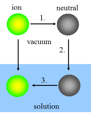
In the Born model, ion solvatation is thought to take place in three steps:
1. Uncharging the ion in vacuum.
2. Bringing the neutral species into the solution.
3. Charging the species in the solution.
The work to charge a species in vacuum is (a = ion radius)
| \( \displaystyle w= \int_{0}^{ze}{V(q)dq}=\int_{0}^{ze}{V \frac{qdq}{4\pi\ \varepsilon _0a}}= \frac{z^2e^2}{8\pi\varepsilon_0a} \), | (2.25) |
|---|
Hence, the work Step 1 has an opposite sign to this. Charging a species in the solution has the work, accordingly
| \( \displaystyle w_3= \frac{z^2e^2}{8\pi\varepsilon_0\varepsilon_ra} \) | (2.26) |
|---|
The electrostatic energy of ion solvation (IS) is therefore
| \( \displaystyle w_{\text{el}}= \Delta G_{\text{IS}}=- \frac{z^2e^2}{8\pi\varepsilon_0a} \left( 1-\frac{1}{\varepsilon_r}\right) \) | (2.27) |
|---|
The work (energy) of Step 2 > 0, because a cavity must be formed for a species in the solution. This work is ~(4/3)πa3P where P is pressure. When a species is brought through the solution surface, work must be done against the surface tension \( \gamma \); that work is \( 4\pi a^2\gamma \).
The electrostatic energy is, however, so dominating and negative that solvation is a spontaneous process. Assume that a = 0.1 nm, z = 1 εr = 78.4, p = 1 atm ja γ = 0.0728 J/m2. The electrostatic energy is now -7.1 eV = -684 kJ/mol, while Step 2 has energy of only 0.057 eV = 5.5 kJ/mol. Although there are other forces in Step 2, we are no longer concerned with them.
If an ion is partitioned between an aqueous and an organic solution, Equation (2.27) can be applied via a thought process where an ion is brought from a vacuum into the both phases. The difference between the solvation energies becomes
| \( \displaystyle w_{\text{el}}= \Delta_o^wG=\pm\frac{z^2e^2}{8\pi\varepsilon_0a} \left( \frac{1}{\varepsilon_r^w} -\frac{1}{\epsilon_r^{o}}\right) \) | (2.28) |
|---|
From Equation (2.11) we see that \( ( \frac{\partial \Delta G}{\partial T})_{p,\mu_i}=-\Delta S \) The entropy of solvation is therefore
| \( \displaystyle \Delta S_{\text{IS}}=- \frac{z^2e^2}{8\pi\varepsilon_0a} \frac{1}{\varepsilon_r^2} \left( \frac{\partial\varepsilon_r}{\partial T}\right) \) | (2.29) |
|---|
Since \( \Delta G=\Delta H-T\Delta S \),
| \( \displaystyle\Delta H_{\text{IS}}=- \frac{z^2e^2}{8\pi\varepsilon_0a} \left( 1-\frac{1}{\varepsilon_r}- \frac{T}{\varepsilon_r^2} \frac{\partial \varepsilon_r}{\partial T}\right) \) | (2.30) |
|---|
For water (∂er/∂T) = -0.3595, giving the enthalpy share of \( \Delta G_{IS} \) -7.2 eV and the entropy share \( -T\Delta S_{IS} \) = +0.1 eV at room temperature. The entropy of solvation therefore increases as a result of issues that are beyond electrostatics. Upon solvation, the solvent molecules are organized around an ion in a configuration that is different from that in the bulk of the solution, reducing the entropy of the solution. These issues are beyond the scope of this book. An interested reader can look at the text book by Y. Marcus [2].
Table 2.1. Standard Gibbs free energy, enthalpy and entropy of ion hydration and the molar volume in water for selected ions. From: Y. Marcus in, A.G. Volkov and D.W. Deamer (Eds.), Liquid/liquid interfaces. Theory and methods, CRC Press, Boca Raton, 1996. With the Publisher’s (CRC Press) permission.
|
|
|
|
|
|
|
|
|
|
|
Cations |
Radius/pm |
\( \Delta G_{hyd}^\theta \) /kJ mol-1 |
\( \Delta H_{hyd}^\theta \) /kJ mol-1 |
\( \Delta S_{hyd}^\theta \) /J mol-1 K-1 |
\( \bar V_m^\theta \) /cm3 mol-1 |
|
|
|
H+ |
|
-1055 |
-1090 |
-131 |
-5.5 |
|
|
|
Li+ |
69 |
-475 |
-530 |
-161 |
-6.4 |
|
|
|
Na+ |
102 |
-365 |
-415 |
-130 |
-6.7 |
|
|
|
K+ |
138 |
-295 |
-330 |
-93 |
3.5 |
|
|
|
Rb+ |
149 |
-275 |
-305 |
-84 |
8.6 |
|
|
|
Cs+ |
170 |
-250 |
-280 |
-78 |
15.8 |
|
|
|
NH4+ |
148 |
-285 |
-325 |
-131 |
12.4 |
|
|
|
Me4N+ |
280 |
-160 |
-215 |
-163 |
84.1 |
|
|
|
Et4N+ |
337 |
-130 |
-205 |
-241 |
143.6 |
|
|
|
Mg2+ |
72 |
-1830 |
-1945 |
-350 |
-32.2 |
|
|
|
Ca2+ |
100 |
-1505 |
-1600 |
-271 |
-28.9 |
|
|
|
Fe2+ |
78 |
-1840 |
-1970 |
-381 |
-30.2 |
|
|
|
Ni2+ |
69 |
-1980 |
-2115 |
-370 |
-35 |
|
|
|
Fe3+ |
65 |
-4265 |
-4460 |
-576 |
-53 |
|
|
|
|
|
|
|
|
|
|
|
|
Anions |
|
|
|
|
|
|
|
|
F– |
133 |
-465 |
-510 |
-156 |
4.3 |
|
|
|
Cl– |
181 |
-340 |
-365 |
-94 |
23.3 |
|
|
|
Br– |
196 |
-315 |
-335 |
-78 |
30.2 |
|
|
|
I– |
220 |
-275 |
-290 |
-55 |
41.7 |
|
|
|
OH– |
133 |
-430 |
-520 |
-180 |
-0.2 |
|
|
|
NO3– |
179 |
-300 |
-310 |
-95 |
34.5 |
|
|
|
ClO4– |
250 |
-205 |
-245 |
-76 |
49.6 |
|
|
|
|
|
|
|
|
|
|
[1] A review of the theory is provided by R.A. Pierotti, Chem. Rev. 76 (1976) 717-726.
[2] Y. Marcus, Ion Solvation, Wiley, 1985.
2.5. Ion-ion interactions
2.5.1 Mean activity coefficient
Activity coefficients of non-electrolytes are close to unity even at moderately concentrated solutions while long-range electrostatic forces between ions mean the activity coefficients of ions must be taken into account even at rather dilute concentrations (c > 1 mM). Ion-ion interaction is traditionally estimated using the Debye-Hückel theory whereby the solvent is taken as a dielectric continuum with a single static relative permittivity \( \varepsilon \)r.
Around an arbitrarily chosen central ion there are more ions with an opposite charge than ions with a like charge.
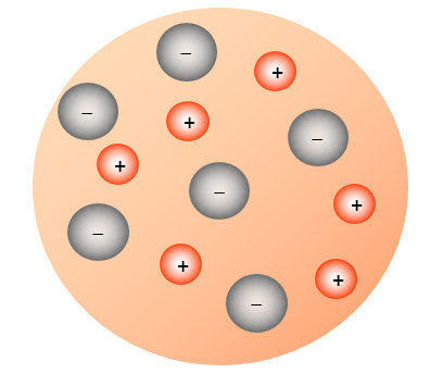
Ions are arranged in the electric field of the central ion according to the Boltzmann distribution:
| \( \displaystyle c_i(r)=c_i^be^{-z_i \phi (r)} \) | (2.31) |
|---|
ci is the concentration of ion i and \( \varphi=F\phi/RT \). Far from the central ion \( \varphi \)(r) = 0, hence ci has its bulk value \( c_i^b \). The charge density \( \rho \)(r) around the central ion is
| \( \displaystyle\rho(r)=\sum\limits_{i}z_iFc_i=\sum\limits_{i}z_iFc_i^be^{-z_i\phi(r)} \approx \sum\limits_{i}z_iFc_i^b\left(1- \frac{z_iF\phi(r)}{RT}\right) =- \frac{F^2\phi(r)}{RT}\sum\limits_{i}z_i^2c_i^b \) | (2.32) |
|---|
It can be shown that the linearization of the exponent is acceptable when c < 0.01 mol/dm3 (T = 298); the last equality comes from electroneutrality in the bulk phase. Inserting the charge density into Poisson equation gives
| \( \displaystyle\nabla^2\phi=- \frac{\rho}{\varepsilon_0\varepsilon_r} \Rightarrow \nabla^2\phi=\kappa^2\phi \) ; \( \kappa^2 \frac{F^2}{\varepsilon_0\varepsilon_rRT}\sum\limits_{i}z_i^2c_i^b \) | (2.33) |
|---|
The quantity \( \kappa \)-1 is known as the Debye length because it bears the length unit. It is a characteristic measure of the thickness of the electric double layer (EDL, Chapter 5), in other words the distance where local electroneutrality does not apply. In an aqueous solution of a 1:1 electrolyte at the 1.0 mM concentration it takes the value of approximately 10 nm (T = 298 K).
The solution of Equation (2.33) in spherical coordinate is (φ(r) = 0 when r → ∞)
| \( \displaystyle r\phi(r)=Ce^{-\kappa r} \) | (2.34) |
|---|
The constant C is solved from the condition that the ion cloud around the central ions compensates its charge zce:
| \( \displaystyle \int_{a}^{\infty }{4\pi r^2\rho(r)dr=-z_ce} \) , | (2.35) |
|---|
Here, a is the distance
of closest approach to the central ion. Using straightforward algebra, the constant C and the potential distribution is obtained as
| \( \displaystyle C=\frac{z_ce} {4\pi\varepsilon_0 \varepsilon_r }\frac{e^{\kappa a}}{1+\kappa a} \Rightarrow \phi(r)=\frac{z_ce} {4\pi\varepsilon_0 \varepsilon_r }\frac{e^{-\kappa(r-a)}}{1+\kappa a}\frac{1}{r} \) | (2.36) |
|---|
Figure 2.3. Scaled potential e−κr as the function of the distance from the central ion at varying concentrations (1-100 mM) of a 1:1 electrolyte; central ion assumed a point charge, a = 0.
In Figure 2.3 above, the potential profiles have been shown as the function of the distance from the central ion. The reference value is the potential created by a single ion
| \( \displaystyle V(r)=\frac{z_ce}{4\pi\varepsilon_0\varepsilon_r}\frac{1}{r} \) | (2.37) |
|---|
The electrostatic work required to bring the central ion into the ion cloud is
| \( \displaystyle w_{\text{ion-ion}}=N_A \int_{0}^{z_ce}{\phi_{\text{atm}}} (a)dq \) ; \( \phi_{\text{atm}}(a)=\phi (a)-V(a)=-\frac{z_ce}{4\pi\varepsilon_0\varepsilon_r}\frac{\kappa}{1+\kappa a}\) | (2.38) |
|---|
| \( \displaystyle w_{\text{ion-ion}}=-\frac{N_A\kappa}{8\pi\varepsilon_0\varepsilon_r}\frac{{(z_ce)^2}}{1+\kappa a} \) | (2.39) |
|---|
When a solution is diluted from concentration c1 to concentration c2, the work of dilution is
| \( \displaystyle w_{\text{dil}}=RT\ln(\frac{a_2}{a_1})=RT\ln(\frac{c_2}{c_1})+RT\ln(\frac{\gamma_1}{\gamma_2})=w_{\text{osm}}+w_{\text{el}} \) | (2.40) |
|---|
Assuming that electrostatic interactions is the root of an activity coefficient, the latter term in the above equation is equal to wion-ion. Since γ2 = 1 (assuming infinite dilution)
| \(\displaystyle \ln\gamma_i=\frac{w_{\text{ion-ion}}}{RT}=-\frac{(z_ce)^2}{8\pi\varepsilon_0\varepsilon_rk_BT}\frac{\kappa}{1+\kappa a} \) | (2.41) |
|---|
It is customary to write Equation (2.41) down with the Briggs logarithm:
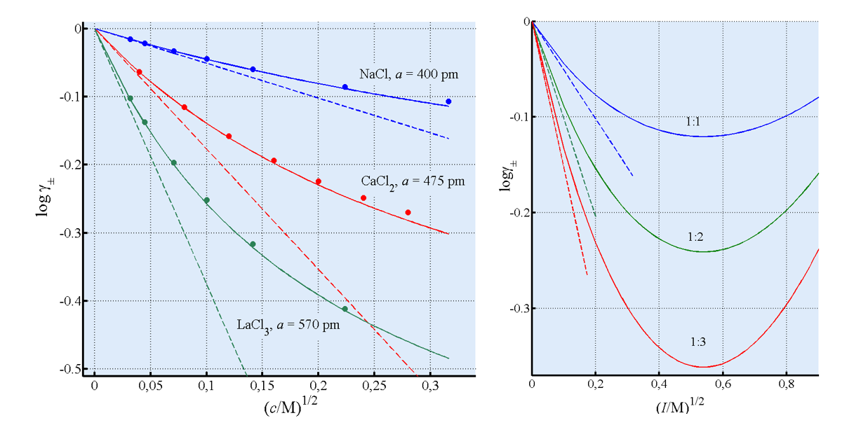
| \( \displaystyle\log\gamma_i=-z_i^2\frac{A\sqrt{I}}{1+Ba\sqrt{I}} \) ; \( I=\frac{1}{2}\sum\limits_{i}z_i^2c_i= \) ionic strength | (2.42) |
|---|
\( \displaystyle A= \frac{1.8246 \cdot10^6 }{(\varepsilon_rT)^{3/2}} \) mol-1/2dm3/2K3/2 ; \( \displaystyle B=\frac{50.29 \cdot10^8}{(\varepsilon_rT)^{1/2}} \) cm-1dm3/2K1/2
Applying the definition of the mean activity coefficient (2.16) the following result is reached:
| \( \displaystyle\log\gamma_{\pm}=z_+z_-\frac{A\sqrt{I}}{1+Ba\sqrt{I}} \) | (2.43) |
|---|
The parameter a is known as the distance of closest approach, the minimum distance between a cation and an anion. In aqueous solutions, the Debye-Hückel model works satisfactorily up to a concentration of 0.1 M. Often only the numerator of Equation (2.43) is used (Debye-Hückel limiting law) if c < 0.01 M. Various more or less empirical equations have been suggested for more concentrated solutions; perhaps the best known is the Davies formula that takes the following form for aqueous solutions at 298 K:
| \( \displaystyle\log\gamma_{\pm}=z_+z_-\frac{0.51\sqrt{I}}{1+\sqrt{I}}-0.20I \) | (2.44) |
|---|
2.5.2 Ion pairing
In solvents with low relative permittivity, ions tend to form ion pairs. Although an electrolyte might dissolve completely in the solvent, it does not dissociate completely into free ions. Dissociation constants can be determined experimentally using, for example, conductivity measurements. The dissociation constant of an electrolyte \( \text{A}_{\upsilon+}B_{\upsilon-} \) , Kd is
| \( \displaystyle K_d=\frac{(\gamma_Ac_A)^{\upsilon_+}(\gamma_Bc_B)^{ \upsilon_-}}{c_{AB}}=\frac{(\alpha\gamma_{\pm})^{\upsilon}c^{\upsilon-1}}{1-\alpha} \) | (2.45) |
|---|
where \( \alpha \) is the degree of dissociation and \( \upsilon=\upsilon_++\upsilon_- \) The activity coefficient of ion pairs is usually taken as unity because they carry no charge. Since α often is rather low, making the ionic strength also low, the mean activity coefficient \( \gamma_{\pm} \) is close to unity. In that case, for a 1:1 electrolyte applies Kd = α2c/(1 - α).
Ion pairing (or ion association) is traditionally analyzed using the theories of Bjerrum or Fuoss. The Bjerrum theory assumes that close to an ion the potential profile is essentially V(r), Equation (2.37). The number of ions i residing in the sphere element of the thickness of dr is therefore
| \( \displaystyle dN_i(r)=4\pi r^2N_i^b\exp(-\frac{z_ieV}{k_BT})dr=4\pi r^2N_i^b\exp(-\frac{z_iz_ce^2}{4\pi\varepsilon_0\varepsilon_rk_BT}\frac{1}{r})dr \) | (2.46) |
|---|
Function (2.46) has a minimum at the point
| \( \displaystyle r=q=\displaystyle\frac{|{z_iz_c|}e^2}{8\pi\varepsilon_0\varepsilon_rk_BT} \) | (2.47) |
|---|
Bjerrum postulated that all ions with the sign opposite to that of the central ion within a distance smaller than q form an ion pair. At the distance q the electrostatic energy of an ion is
| \( \displaystyle\frac{|{z_iz_c|}e^2}{4\pi\varepsilon_0\varepsilon_rq}=2k_BT \) | (2.48) |
|---|
The fraction of paired (associated) ions, 1 - α, is therefore
| \( \displaystyle 1-\alpha= \int_{a}^{q}{dN_i(r)dr} =4\pi N_i^b \int_{a}^{q}{r^2e^{2q/r}dr} \) | (2.49) |
|---|
With the change of variables x = 2q/r the above equation can be written in the form of
| \( \displaystyle 1-\alpha=4\pi N_i^b \cdot(2q)^3 \int_{2}^{b}{x^{-4}e^xdx} \) ; \( b=\frac{2q}{a}=\frac{|{z_+z_-|}e^2}{4\pi\varepsilon_0\varepsilon_rak_BT} \) | (2.50) |
|---|
The integral (Bjerrum integral) in the above equation must be evaluated numerically. The ion-pairing (association) constant Ka (= 1/Kd) is relatively easy to calculate. Assume an ion-pairing reaction A+ + B- ↔ AB. Now, from Equation (2.45)
| \( \displaystyle K_a=\frac{1-\alpha}{\alpha^2c}\frac{\gamma_{\text{AB}}}{\gamma_{\pm}^2} \) | (2.51) |
|---|
Because Ka is the same at each concentration, in a very diluted solution where α ≈ 1 and \( \gamma_{\pm} \) ≈ 1, Ka ≈ (1 - α)/c. Inserting Equation (2.50) into this and changing the species number density Nib (m-3) to the molar concentration gives
| \( \displaystyle K_a=4000\pi N_A(\frac{|{z_iz_c|}e^2}{8\pi\varepsilon_0\varepsilon_rk_BT})^3 \int_{2}^{b}{x^{-4}e^xdx} \) | (2.52) |
|---|
where NA is the Avogadro number, 6.023×10²³ mol-1. The weakest point in the Bjerrum theory is its rather arbitrary choice q = 2kBT. For a 1:1 electrolyte in water at room temperature (298 K) the value of Ka is ca. 1.27 dm3/mol (a = 0.2 nm), proving that common electrolytes do not make ion pairs in water to a significant extent.
The Fuoss theory presumes contact between ions in order to form an ion pair. Let’s consider again a 1:1 electrolyte. Let the number of free ions in the solution be N+ = N- = N1 and N2 the number of ion pairs. After adding δN anions and cations in the solution a fraction of them remains free and a fraction makes ion pairs. The probability that an anion remains free is proportional to the amount of δN added and to the volume that is not occupied by cations:
| P(free) \( \displaystyle \sim(V-N_1 \nu_+) \delta N \) | (2.53) |
|---|
where V
is the total solution volume and ν+
the volume of a cation. Accordingly, the probability that an anion makes an ion
pair is, in addition to space occupied by cations, N1v+, and to the added amount, δN also proportional to the Boltzmann factor e-E(a)/kBT:*
| P(ion pair) \( \displaystyle \sim N_1\nu_+e^{-E(a)/k_BT} \delta N \) | (2.54) |
|---|
The electrostatic energy of an anion in contact with a cation, E(a) is obtained from Equation (2.37). Let the number of anions that make an ion pair be δN2 and the number of anions remaining free δN1. A similar analysis can of course be done for cations. Due to electroneutrality, the number of cations that make ion pairs must also be δN2, making the total number ion pairs 2δN2. Probabilities are proportional to the numbers. Therefore,
| \( \displaystyle\frac{\delta N_2}{\delta N_1}=\frac{2N_1 \nu_+e^{-E(a)/k_BT}dN}{(V-N_1 \nu_+)dN } \) | (2.55) |
|---|
Assuming that the solution is so dilute that the volume occupied by cations, N1v+, is insignificant with respect to the solution volume V, Equation (2.55) can be integrated with respect to N1. The result is of course
| \( \displaystyle N_2=N_1^2e^{E(a)/k_BT}\nu_ +/V \) | (2.56) |
|---|
The concentration of free ions, N1/V, is in terms of molarity
| \( \displaystyle N_1/V= \alpha cN_A \cdot1000 \) | (2.57) |
|---|
Accordingly, the concentration of ion pairs is
| \( \displaystyle N_2/V=(N_1/V)^2e^{-E(a)/k_BT}(4/3)\pi a^3=(1- \alpha)cN_A \cdot1000 \) | (2.58) |
|---|
Combining Equations (2.51), (2.57) and (2.58) the following formula is reached:
| \( \displaystyle\frac{1-\alpha}{\alpha^2c}=1000N_A(\frac{4}{3}\pi a^3)e^{-E(a)/k_BT} \) | (2.59) |
|---|
The mean activity coefficient is again assumed to be unity due to the dilute concentration.
2.5.3 Super acids and Hammett acid function[1]
In very strong acids, such as in pure sulphuric acid or in its mixtures with organic solvents, ion association and activity coefficients become rather ambiguous quantities. Yet it has been experimentally demonstrated that these kinds of solutions are very acidic, having a negative pH: they are called super acids. Analogously, mixtures of strong bases with organic solvents are vary basic, having a pH beyond the scale of ordinary pH sensors because they can make the sensor unstable or even destroy it.
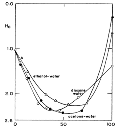
For the analysis of super acids and bases, Hammett introduced an acid function H0 that can be considered to be an extension of the common pH scale. In order to determine the value of H0, a weak indicator base B is added to the super acid solution, and the concentration of B is determined with, for example, UV spectrophotometer. The base protonates to BH+, and its dissociation equilibrium is
| BH+ \(\ce{ <=> }\) B + H+ | (2.60) |
|---|
The equilibrium constant is of course
| \( \displaystyle K_d=\frac{a_{H^+}a_B}{a_{BH^+}} \) | (2.61) |
|---|
Taking the negative of the Briggs logarithm as usual
| \( \displaystyle pK_d+\log\frac{[B]}{[BH^+]}=-\log(a_{H^+})-\log\frac{\gamma_B}{\gamma_{BH^+}} \equiv H_0 \) | (2.62) |
|---|
Equation (2.62) defines the Hammett acid function H0 that can be experimentally defined because the concentration ratio [B]/[BH+] can be measured with spectroscopy. For example, for water-free suphuric acid H0 = -12.0. Nitroanilines are typical indicator bases. The values of their equilibrium constants (Kd) in solvents other than water pose a problem of its own that must be solved with various means of comparison and extrapolation6.
In alkaline solutions the corresponding function is H− that corresponds to the equilibrium
| BH + OH−(H2O)n \(\ce{ <=> }\) B− + (n + 1)H2O ; | (2.63) |
|---|
where n is the hydration number of the hydroxide ion. In pure water its value is approximately 5.5. In aqueous solutions the function H− can be estimated with the equation
| \( H_-=pK^w+\log[OH^-]-(n+1)\log[H_2O] \) | (2.64) |
|---|
In Equation (2.64), Kw is the ionic product of water and [H2O] is the concentration of free water in the solution. Their values naturally depend on the solution composition.
* When an anion approaches a cation E(a) is the energy released in the process. The Boltzmann factor is also found in the Grand Canonical partition function of ion binding.
[1] M.A. Paul, F.A. Long, ’H0 and related indicator acidity functions’, Chem. Rev. 57 (1957) 1-45.
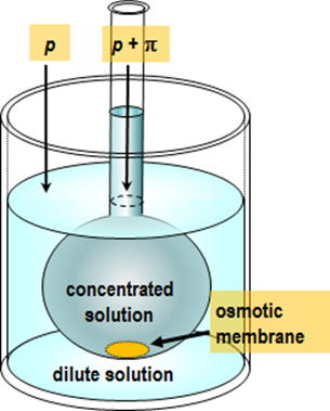
2.6. Osmosis
When a semi-permeable membrane separates two electrolyte solutions of different concentrations, osmotic pressure is created across the membrane. It should be emphasized that an ideal osmotic membrane is not permeable to any species other than water. Osmotic pressure is formed across an ion-selective membrane, but since no real membrane is ideal, the tiny amount of co-ions* in the membrane allows for slow diffusion of salt across the membrane, ultimately dissipating osmotic pressure. In biology, osmosis is an important issue but a cell membrane is not, strictly speaking, an osmotic membrane. Ionic concentrations are maintained by active membrane transporters.
Despite of the above critical comments, let us consider the emergence of osmotic pressure across an ideal osmotic membrane. Osmotic pressure is formed due to the imbalance of the chemical potential of water. Because only water can cross the membrane, the equilibrium condition of water at a constant temperature (dT = 0) between two aqueous phases α and β is written as
| \( \displaystyle\mu_1^{\alpha}\left(p,x_i^{ \alpha}\right)= \mu_1^{\beta}\left(p,x_i^{ \beta}\right) \) | (2.65) |
|---|
The chemical potential of water is therefore a function of the concentrations of all species and the pressures of the phases. (Subscript ’0’ is reserved for the solvent and the others for solutes.) The pressure dependence of the chemical potential is obtained using Equations (2.6) and (2.11) (note that the order of differentiation is free):
| \( \displaystyle\left(\frac{\partial\mu_i}{\partial p}\right)=\frac{\partial}{\partial p}\left(\frac{\partial G}{\partial n_i}\right)=\frac{\partial}{\partial n_i}\left(\frac{\partial G}{\partial p}\right)=\left(\frac{\partial V}{\partial n_1}\right)=\overline{V}_i \) | (2.66) |
|---|
where \( \overline{V_i} \) is the partial molar volume of species i. On the mole fraction scale
| \( \displaystyle d\mu_1=RTd\ln(f_1x_1)+\overline{V_1}dp \Rightarrow \mu_1=\mu_1^0+RT\ln(f_1x_1)+\overline{V_1}p \) | (2.67) |
|---|
Equation (2.67) is formally reached by an integration between pure water and a solution with the mole fraction x0 and activity coefficient f0 of water. Equilibrium between phases \( \alpha \) and \( \beta \) is therefore
| \( \displaystyle RT\ln(f_1^{\alpha}x_1^{\alpha})+\overline{V_1}^{\alpha}p^{\alpha}=RT\ln(f_1^{\beta}x_1^{\beta})+\overline{V_1}^{\beta}p^{\beta} \) | (2.68) |
|---|
Water is incompressible, and therefore its partial molar volume is constant unless the concentrations in the two solutions are very different. Osmotic pressure is:
| \( \displaystyle\pi=p^{\alpha}-p^{\alpha}=-\frac{RT}{\overline{V_1}}\ln\left(\frac{f_1^{\alpha}x_1^{\alpha}}{f_1^{\beta}x_1^{\beta}}\right) \approx-\frac{RT}{\overline{V_1}}\ln\frac{x_1^{\alpha}}{x_1^{\beta}} \) | (2.69) |
|---|
The ratio of the actitivy coefficients ≈ 1. Assume that phase β is pure water. Then
| \( \pi \approx -\frac{RT}{\overline{V_1}}\ln(x_1)=\frac{RT}{\overline{V_1}}\ln\left(1-\sum\limits_{k\neq1}x_k\right) \approx\frac{RT}{\overline{V_1}}\left(\sum\limits_{k \neq1}x_k\right) \) | (2.70) |
|---|
Because xk « x0 ≈ 1, xk ≈ nk /n0, and \( \overline V_1n_1 \approx V \) is the volume of the solution,
\( \pi \approx RT \sum\limits_{k}c_k \) |
(2.71) |
|---|
Equation (2.71) is known as the Van’t Hoff equation. Inserting, for example, c = 1.0 M = 1000 mol/m3, we see that \( \pi \) ≈ 24.5 atm (T = 298 K) corresponding to approximately 250 m height of a water column. This has led to the idea of a power plant that would harness osmotic pressure. An osmotic membrane is, however, very dense, making the flux of water very low. The power density hence remains very low, which makes such a power plant commercially unviable.
Equation (2.70) can be improved with an osmotic coefficient
| \( \displaystyle\pi=-\frac{RT}{\overline{V}}\ln(f_1x_1)=-\frac{\Phi RT}{\overline{V_1}}\ln (x_1) \Rightarrow \Phi-1=\frac{\ln f_1}{\ln x_1} \) | (2.72) |
|---|
that takes the unideality of a solution into account. Its values are tabulated for common electrolytes.
The correlation between the mean activity coefficient of an electrolyte and the osmotic coefficient is given without derivation in a binary system with the concentration c:
| \( \displaystyle d(c\Phi)=dc+c d\ln(\gamma_\pm) \Rightarrow\Phi=1+\frac{1}{c} \int_{0}^{c}{cd\ln\gamma_{\pm}} \) | (2.73) |
|---|
| \( \displaystyle d\ln\gamma_{\pm}=d\Phi+(\Phi-1)d\ln c \Rightarrow\ln\gamma_{\pm}=(\Phi-1)+ \int_{0}^{c}{(\Phi-1)} d\ln c \) | (2.74) |
|---|
If γ± is known in the concentration range [0,c], Φ can be calculated from Equation (2.73).
Accordingly, if the osmotic coefficient is measured in the same range, γ± can be calculated from (2.74). Measuring the mean activity coefficient
is relatively easy using electrochemical methods (electromotive force of a Galvanic
cell), and the osmotic coefficient can be evaluated from an experiment with an
osmometer; the principle of such an experiment is depicted in Figure 2.6.
The Van’t Hoff equation can also be used to determine the molar mass of a macromolecule. Inserting a sample with mass m into the measurement chamber with the volume V, and measuring osmotic pressure, the molar mass M is obtained from the formula
| \( \displaystyle M=\frac{mRT}{\pi V} \) | (2.75) |
|---|
In biological experiments it is important to keep solutions isotonic, i.e. their osmocity equal to that of a living cell. Osmocity S is defined as the concentration of NaCl solution that has the same freezing point \( \Delta \)Tf as the solution being investigated. Osmolality O = ΔTf /Kf (Os/kg water) where Kf is the cryoscopic constant. ΔTf = -Kf m where m is the molality of a solute (≈ c). For water Kf = 1.86. The relation between the freezing point depression and osmotic pressure is (T = 273 K)
| \( \displaystyle\frac{\pi}{\text{atm}}=RT\frac{\Delta T_f}{K_f}=\frac{22.4}{1.86} \Delta T_f \cong12 \Delta T_f \) | (2.76) |
|---|
Equation (2.76) can be improved to also include the second term of the series expansion of Equation (2.70). In that case,
| \( \displaystyle\pi\cong12\Delta T_f-0.021(\Delta T_f)^2 \) atm | (2.77) |
|---|
Table 2.2 shows a few constants of freezing point depression and boiling point elevation for selected molecules; ΔTb = Kb m.
Table 2.2. Constants of freezing point depression and boiling point elevation for selected molecules. From: Handbook of Chemistry and Physics, 83. p. CRC Press, Boca Raton, 2002. With Publisher’s permission (CRC Press).
|
Substance |
Normal freezing point (K) |
Kf (K kg mol–1) |
Normal boiling point (K) |
Kb(K kg mol–1) |
|
Acetic acid |
289.6 |
3.59 |
391.2 |
3.08 |
|
Benzene |
278.6 |
5.12 |
353.3 |
2.53 |
|
Camphor |
449 |
40 |
482.3 |
5.95 |
|
Carbon disulfide |
161 |
3.8 |
319.2 |
2.40 |
|
Carbon tetrachloride |
250.3 |
30 |
349.8 |
4.95 |
|
Cyclohexane |
279.6 |
20.0 |
353.9 |
2.79 |
|
Ethanol |
158.8 |
2.0 |
351.5 |
1.07 |
|
Phenol |
314 |
7.27 |
455.0 |
3.04 |
|
Water |
273.15 |
1.86 |
373.15 |
0.51 |

| Example: The freezing point of blood serum is -0.53 °C. From Equation (2.77) we can calculate that its osmotic pressure \( \pi \) = 12.06×0.53 - 0.021×(0.53)2 atm ≈ 6.39 atm. The freezing point depression corresponds to approximately 0.53/1.86 ≈ 0.285 mol/kg NaCl solution. If a solution that is isotonic with serum is made from glucose, the glucose concentration should be approximately 88 g/dm3. Urea is frequently used in biochemistry: its required concentration would be only approximately 32 g/dm3 (values from the CRC table). The freezing point of a physiological solution (0.15 mol/kg NaCl) would be -0.28 °C, if calculated from the above equations. |
|---|
Quantities introduced in this paragraph are all colligative properties, i.e. the nature of the dissolved species does not, in principle, matter, only their concentration. A careful reader will note that osmotic coefficients are different for different electrolytes, which conflicts with the definition of the colligative properties. The theory presented above therefore only applies at moderately low concentrations.
* An ion with the opposite charge of the membrane is a counter-ion and an ion with the same charge a co-ion.
You can now test your conceptual knowledge by taking Quiz Chapter 2
3. Transport in electrolyte solutions
In the Introduction of this book, we explained that the analysis of transport processes in electrolyte solutions constitutes the salient part of electrochemistry. Because electric current can occur only in a closed circuit, it also flows across the electrolyte solution that contributes to the properties of an electrochemical cell. More importantly, transport of electroactive species provides the boundary condition for the solution of electrochemical problems, as will be seen later.
From the point of view of transport, an electrolyte solution can be roughly divided into two domains: the interior or the bulk solution and the polarization layer close to the electrode surface. The bulk solution is chemically homogeneous, merely determining the total resistance of the cell via its conductivity. The thickness of the polarization layer is of the order of a few microns where concentration changes take place. These changes are due to electrode reactions. Let us consider a simple one-electron transfer reaction
| Cu2+ + e - \(\ce{ <=> }\) Cu+ , | (3.1) |
|---|
where Cu2+ reduces to Cu+. As the reaction occurs on the electrode surface, the concentration of Cu2+ on the surface (x = 0) decreases and that of Cu+ simultaneously increases. Transport, in other words diffusion (and migration) tries to compensate for the emerging deficit of Cu2+ and excess of Cu+. The reaction rate, r, is a scalar while the flux of a species, J, is a vector although they both have the unit mol cm2 s-1. These two quantities with different tensorial dimensions are coupled via the mass balance and the Faraday law:
| \(\displaystyle r=- \frac{i}{F}=-J_{\text{Cu}^{2+}}|_{x=0}=J_{\text{Cu}^+}|_{x=0} \) | (3.2) |
|---|
Equation (3.2) shows that an electrode reaction, i.e. electric current density, is the boundary condition of a transport problem. This is the specific feature – and the mathematical difficulty – of electrochemical analysis. In an electrochemical experiment, electric current, the boundary condition of a transport problem, is usually measured, not the concentration that is the quantity appearing in the transport equations. This means there is a need for the evaluation of concentration (and potential) gradients at the surface. Often numerical methods must be resorted to in order to solve a transport problem, and the calculation of numerical derivatives is prone to errors in accuracy.
The surface concentrations \( c_i^s \) adjust themselves so that the reaction rate equals to the rate of transport:
| \( \displaystyle r=k_{\text{red}}c_{\text{Cu}^{2+}}^s-k_{ox}c_{\text{Cu}^{+}} \) | (3.3) |
|---|
where kred and kox are the reaction rate constants of reduction and oxidation respectively. If a reaction is very fast, i.e. reversible, its rate is limited by the transport of the reactant to the electrode. In that case the surface concentrations are coupled with the Nernst equation instead of Equation (3.3), but in all cases Equation (3.2) must be applied in the analysis.
3.1. Conductivity of an electrolyte solution
Let’s consider the situation in Figure 3.1: a particle (ion) with the charge q = ze feels a coulombic force \( F_c \) in an electric field E:
| \( F_c=qe=zeE \). | (3.4) |
|---|
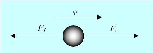
The coulombic force makes the particle move with the velocity v (no vector notation):
| \( v=uE \), | (3.5) |
|---|
where u is the mobility of the particle. Friction resists the movement:
| \( F_f=-fv \) | (3.6) |
|---|
In Equation (3.6) Ff is the frictional force and f the friction coefficient for which Einstein derived an expression
| \( \displaystyle f= \frac{kT}{D} \) | (3.7) |
|---|
At equilibrium, the friction
force and the coulombic force cancel each other out, and we get:
| \( \displaystyle zeE= \frac{kT}{D}v \Leftrightarrow v=\frac{zeD}{kT}E=\frac{zFD}{RT}E \). | (3.8) |
|---|
Comparing Equation (3.5) with (3.8) it is immediately seen that
| \( \displaystyle u= \frac{zFD}{RT} \). | (3.9) |
|---|
It is easy to prove that a particle reaches constant velocity immediately after switching on the electric field. Newton’s second law can be written in the form
With the initial condition v(t = 0) = 0 the solution is
Inserting typical values of the quantities into the above equation, we see that the exponential (f/m) is of the order of 109 s-1, i.e. the relaxation time is of the order of nanoseconds. |
|---|
Electric current density i is defined using the Ohm’s law:
| \( i= \kappa E \) | (3.12) |
|---|
where \( \kappa \) is the conductivity of the solution. It can be written as the sum of the product of molar conductivities, \( \lambda \)k, and concentrations, ck, of all ions:
| \( \displaystyle\kappa =\sum\limits_{k}\lambda_kc_k \) | (3.13) |
|---|
| \( \displaystyle i=F\sum\limits_{k}z_kJ_k=F\sum\limits_{k}z_kv_kc_k \) | (3.14) |
|---|
Inserting Equation (3.8) into (3.14), the following is obtained:
| \( \displaystyle i= \frac{F^2}{RT}\sum\limits_kz_k^2D_kc_k \cdot E \) | (3.15) |
|---|
| \( \displaystyle\lambda_k= \frac{F^2z_k^2D_k}{RT} \) | (3.16) |
|---|
The relation between uk and \( \lambda \)k is
| \( \lambda_k=z_ku_kF \) | (3.17) |
|---|
The above equation means that the mechanical and electrical mobility are assumed to be equal. Stokes' law defines the friction coefficient of a spherical object as
| \( f=6\pi\eta a \) | (3.18) |
|---|
where η is the viscosity of the solution and a is the particle radius. Quite surprisingly, Stokes' law applies also to ions although they are of the same order of magnitude as solvent molecules, and although the law was derived via hydrodynamic considerations for macroscopic objects moving in a homogeneous medium. Assuming a as the ion radius, it follows from Equation (3.7) that
| \( \displaystyle D= \frac{kT}{6\pi\eta a} \) | (3.19) |
|---|
Multiplying this equation by η, only solvent independent constants are left on the right hand side: we have derived Walden's rule:
| \( D\eta= \)constant | (3.20) |
|---|
Walden's rule can be used to estimate the values of diffusion coefficients in solvents where there is no measured data. The rule does not, however, apply particularly well to ions in aqueous solutions due to their strong hydration (see Figure 3.2).
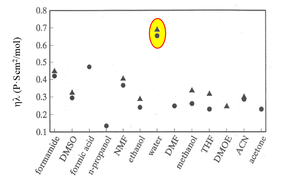
Figure 3.2. The product \( \eta\ \lambda_i \) for K+ (●) and Cs+ (■) cations in selected solvent: DMSO = dimethyl sulphoxide, NMF = n-methyl formamide, DMF = dimethyl formamide, THF = tetrahydrofurane, DMOE = dimethoxy ethane, ACN = acetonitrile. Note water! A.K.Kontturi et al., Ber. Bunsenges. Phys. Chem. 99 (1995) 1131. (P = poise = 0.1 Ns/m2).
3.2. Concentration dependence of conductivity
The conductivity of a solution depends on the ionic concentrations, radii and viscosity of the solvent. Measuring the conductivity of the solution thus is – in principle – a simple means to determine ionic concentrations if molar conductivities are known, but there are a couple of problems. First, the above theory only concerns interactions between ions and solvent, i.e. it is valid in dilute solutions only. Second, an ionic radius in a solution is not an unambiguous quantity due to ion solvation. For example, the mobility of Li+ in water is lower than that of Na+, although its crystallographic radius is smaller. This is because Li+ is so strongly hydrated that it drags a mantle of water with it during transport. Polyatomic ions such as sulphate are not completely spherical either.
Nevertheless, measuring conductivity is one of the oldest electrochemical measurements, and data is available for common electrolytes in a wide range of concentrations and temperatures in aqueous solutions. The division of electrolytes into strong and weak ones, and classical theories of electrolytes are based on this experimental data.
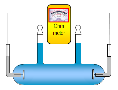
Conductivity is measured with AC current in order to prevent concentration polarization. The electrodes are usually porous platinum plates to minimize the resistance that may occur as a result of electrode reactions. The measured resistance of a conductivity cell (Figure 3.3), Rs is
| \( \displaystyle R_s= \frac{1}{\kappa} \frac{l}{A} \) | (3.21) |
|---|
The geometric cell constant A/l is evaluated using a solution with known conductivity, usually 1.0 mM KCl.
3.2.1 Strong electrolytes
Ion-ion interaction is very strong compared with other intermolecular forces. It is inversely proportional to distance while, van de Waals interaction, for example, is inversely proportional to the sixth power of distance. Typical electrostatic energy between two ions can be as high as 250 kJ mol-1, which is of the order of the energy of a covalent bond, while the energy of a hydrogen bond is only approximately 10-40 kJ mol-1. Coulombic forces may cause some extra trouble in molecular dynamics simulations of electrolytes because it is not sufficient to compute the interactions with the neighboring molecules only but computation must be extended over several layers of molecules. Periodical boundary conditions are often needed because electrostatic forces can stretch over the limits of the simulation domain.
Due to coulombic interactions the activity coefficients of electrolytes deviate from unity even in rather dilute solutions. For the same reason, ionic molar conductivity also very much depends on the concentration. The concentration dependence of a diffusion coefficient is obtained as (see paragraph 3.3)
| \( \displaystyle D_i=D_{i,\infty}\left(1+ \frac{\partial\text{ln}\gamma_i}{\partial\text{ln}c_i}\right) \) | (3.22) |
|---|
where Di,∞ is the diffusion coefficient at infinite dilution. The dependence of an activity coefficient on the concentration is given by the Debye-Hückel theory. Using the limiting law
| \( \text{log}\gamma_{\pm}=z_+z_- A\sqrt{I} \) | (3.23) |
|---|
For a 1:1 electrolyte (I = c = ci):
| \( \displaystyle \frac{\partial\text{ln}\gamma_i}{\partial\text{ln}c_i}=c\frac{\partial\text{ln}\gamma_i}{\partial c}=- \frac{1}{2}A \sqrt{c} \) | (3.24) |
|---|
| \( \displaystyle D_i=D_{i, \infty}\left(1- \frac{2.303}{2}A \sqrt{c}\right) \) | (3.25) |
|---|
Molar conductivity of an electrolyte,
Λ, is the sum of ionic conductivities,
| \( \Lambda= \upsilon_+\ \lambda_++ \upsilon_-\ \lambda_- \). | (3.26) |
|---|
Hence, combining Equations (3.16), (3.25) and (3.26) Kohlrausch's law is achieved,
| \( \Lambda= \Lambda_{ \infty}-K\sqrt{c} \), | (3.27) |
|---|
which is experimentally verified in relatively dilute solutions (c < 0.1 M). Since K includes the product z+z− it is the same for all salts of the same type, see Figure 3.4. Measuring \( \Lambda \) at varying concentrations and extrapolating to infinite dilution, \( \Lambda_ \infty \)can be determined. Combining this data with transport numbers that are discussed later on, ionic molar conductivities at infinite dilution, λi,∞, can be evaluated. Tables of these can be found in several textbooks of physical chemistry.
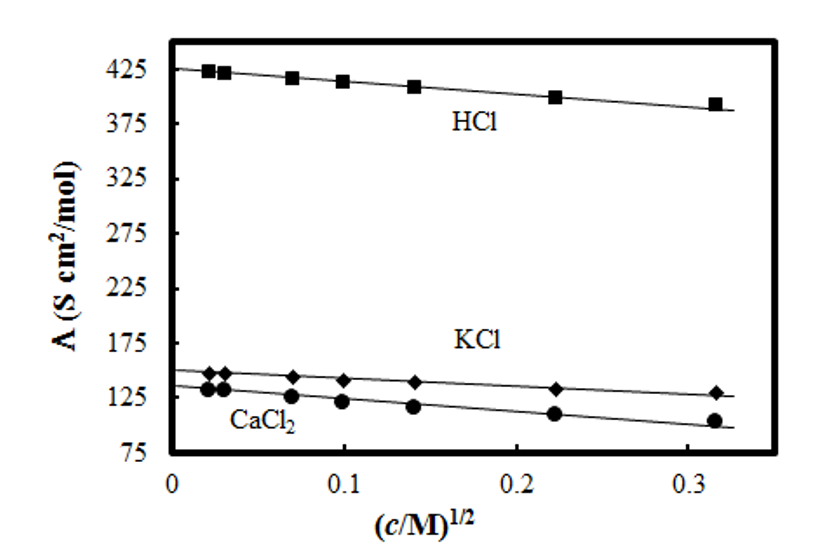
3.2.2 Weak electrolytes
The conductivity of weak
electrolytes that only partially dissociate to free ions follows a different kind
of dependence on the concentration (see paragraph 2.5.2 for a discussion of
dissociation). Since the degree of dissociation, \( \alpha \), is often quite low, the concentrations of free
ions also remain low, and their molar conductivities are practically equal to
the values at infinite dilution. For a 1:1 electrolyte the conductivity \( \kappa \) is
| \( \kappa= \alpha c( \lambda_{+, \infty}+ \lambda_{-, \infty})=\alpha c \Lambda_{ \infty} \) | (3.28) |
|---|
and therefore
| \( \displaystyle \alpha= \frac{\Lambda}{\Lambda_ \infty} \) | (3.29) |
|---|
Arranging the expression of the dissociation constant Kd = α2c/(1 – α) in the form of
| \( \displaystyle\frac{1}{\alpha}=1+\frac{\alpha c}{K_d} \Rightarrow \frac{1}{\Lambda}=\frac{1}{\Lambda_{\infty}}+\frac{\Lambda c}{K_d\Lambda_\infty^2}\) | (3.30) |
|---|
a plot of Λ-1 vs. Λc = κ is linear with the intercept \( \Lambda_ \infty^{-1} \) on the y axis; Kd can be calculated from the slope. Equation (3.30) is known as Ostwald's dilution law; it applies relatively well in aqueous solutions.
In organic solvents, electrolyte dissociation is nearly always incomplete. Constants A and B in the Debye-Hückel theory include the relative permittivity of the solvent εr (previously called the dielectric constant). Calculating their values it transpires that even at low ionic strengths (c < 10-3 M) the mean activity coefficient deviates from unity. Ostwald's dilution law therefore does not apply as such but the activity coefficients need to be retained in the analysis.
Molar conductivity can be written in the form of (1:1 electrolyte)
| \( \Lambda=\alpha(\Lambda_\infty-K\sqrt{\alpha c}) \) | (3.31) |
|---|
Solving \( \alpha \) from the expression of Kd (Equation (2.45)) gives:
| \( \displaystyle\alpha=\frac{K_d(\sqrt{1+4\gamma_{\pm}^2c/K-d}-1}{2\gamma_{\pm}^2c} \) | (3.32) |
|---|
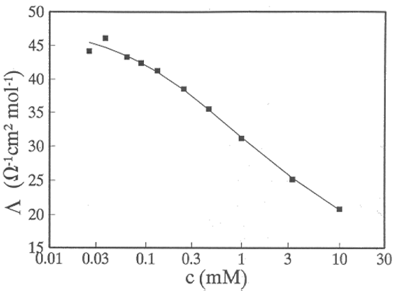
[1] Large number conductivity measurements in varying solution composition with the above analysis is given by R.M. Fuoss et al., J. Soln. Chem. 3 (1974) 45; 4 (1975) 91; 4 (1975) 175.
3.3. Transport equation in a steady state
Transport processes can be approached in various theoretical ways. The most traditional theory is thermodynamics of irreversible processes. In this book we use the most practical means, the Nernst-Planck equation. We bypass the simplifying approximation with which the Nernst-Planck equation can be derived from the theory of irreversible thermodynamics. The Nernst-Planck equation expresses an ionic flux, Jk (mol cm2 s-1), as the sum of three contributions:
| \( \displaystyle\vec{J}_k=-D_k\nabla c_k-\frac{z_kF}{RT}D_kc_k\nabla \phi+\vec{v}c_k \) | (3.33) |
|---|
The first term of Equation (3.33) relates to diffusion, the second one to migration and the third one to convection. The first term alone is equal to Fick’s first law stating that concentration differences tend to level out due to Brownian movement. The second term describes the movement of a charged species in an electric field, in other words electrophoresis. The velocity \( \vec{v} \) found in the convection term is practically equal to the solvent velocity. Convection comes from stirring the solution (forced convection) or density gradients formed in the solution (natural convection).
In the bulk solution no concentration gradients are usually found and, therefore, transport takes place only as a result of migration and convection or, in the absence of stirring, plain migration. In the polarization layer, diffusion plays the main role because, depending on the viscosity of the solvent, an unstirred stagnant hydrodynamic layer is formed on the surface of the electrode. Inert electrolytes that do not react on the electrode are usually added in an electrochemical cell. Such an electrolyte is commonly called as a supporting electrolyte because it carries most of electric current. As a consequence, the flux of an electroactive species is in practice solely diffusion; more detailed evidence is provided later on. In the absence of a supporting electrolyte, the mathematical analysis of transport becomes rather complex and the ohmic losses in the cell may grow in an uncontrollable way.
Equation (3.34) can be written in a compact form with the gradient of electrochemical potential:
| \( \vec{J}_k=-L\nabla \tilde{\mu}_k \), | (3.34) |
|---|
where L is known as the phenomenological coefficient. Inserting the expression of \( \tilde{\mu}_k \), Equation (2.7) here, the following is obtained
| \(\displaystyle \vec{J}_k=-L(RT\nabla \text{ln}c_k+RT\nabla \text{ln} \gamma_k+z_kF \nabla \phi) \) | (3.35) |
|---|
Comparing the
above equation with the Nernst-Planck equation it is seen that [1]
| \( \displaystyle L=\frac{D_kc_k}{RT} \) | (3.36) |
|---|
| \(\displaystyle \vec{J}_k=-D_k \nabla c_k(1+\frac{\partial \text{ln} \gamma_k}{\partial \text{ln} c_k})-\frac{z_kF}{RT}D_kc_k\nabla \phi \) | (3.37) |
|---|
If the dependence of the activity coefficient on concentration is omitted, the first two terms of the Nernst-Planck equation are thus obtained. The convection term comes from the notion that flux can always be written in the form \( \vec{J}_k=c_k \vec{v}_k \) and interpreting \( \vec{v} \) as the solvent velocity.
[1] Equation (3.36) does not apply in general. See, e.g. Kontturi et al., Ionic Transport Processes, Oxford University Press, 2nd Ed. 2015.
3.4. Analysis of transport equations in a steady state
The Nernst-Planck equation must be written out for each species in the solution. Constraints of the group of equations are the electroneutrality condition and electric current density:
| \( \displaystyle\sum\limits_{k}z_kc_k=0 \) | (2.3) |
|---|
| \(\displaystyle i=F\sum\limits_{k}z_kJ_k \) | (3.14) |
|---|
The solution of the group is possible in closed form,2 but let us highlight a couple of its important features with the help of a binary electrolyte \( A_{\upsilon_+}B_{\upsilon_-} \). Division by diffusion coefficients gives
| \( \begin{cases}-\displaystyle\frac{J_+}{D_+}=\nabla c_{+}+\displaystyle\frac{z_+F}{RT}c_+\nabla\phi-\displaystyle\frac{v}{D_+}c_+ \\ -\displaystyle\frac{J_-}{D_-}=\nabla c_{-}+\displaystyle\frac{z_-F}{RT}c_-\nabla\phi-\displaystyle\frac{v}{D_-}c_-\end{cases} \) | (3.38) |
|---|
Ionic concentrations are c+
= \( \upsilon \)+c and c- = \( \upsilon \)-c, and the condition of electroneutrality can be written as z+\( \upsilon \)+ + z-\( \upsilon \)- = 0. Summing above equations, \( \nabla\phi \) is eliminated:
| \( \displaystyle\frac{J_+}{D_+}-\frac{J_-}{D_-}=(\upsilon_++\upsilon_-)\nabla c-\left(\frac{\upsilon_+}{D_+}+\frac{\upsilon_-}{D_-}\right)vc \) | (3.39) |
|---|
With equation (3.14) and electroneutrality, the left had side of Equation (3.39) can be written as
| \(\displaystyle -J_+\left(\frac{1}{D_+}-\frac{z_+}{z_-D_-}\right)-\frac{i}{z_-D_-F}=-J_+\left(\frac{1}{D_+}+\frac{\upsilon_-}{\upsilon_+D_-}\right)-\frac{i}{z_-D_-F} \) |
(3.40) |
|---|
and equation (3.38) using straightforward algebra:
| \( \begin{cases}J_+=-\displaystyle\frac{(\upsilon_++\upsilon_-)D_+D_-}{\upsilon_-D_++\upsilon_+D_-}\nabla c_++\frac{D_+}{z_+D_+-z_-D_-}\displaystyle\frac{i}{F}+vc_+\\J_-=-\displaystyle\frac{(\upsilon_++\upsilon_-)D_+D_-}{\upsilon_-D_++\upsilon_+D_-}\nabla c_--\displaystyle\frac{D_-}{z_+D_+-z_-D_-}\displaystyle\frac{i}{F}+vc_-\end{cases} \) | (3.41) |
|---|
The coefficient of the concentration gradient is the electrolyte diffusion coefficient D±:
| \( \displaystyle D_{\pm}=\frac{(\upsilon_++\upsilon_-)D_+D_-}{\upsilon_-D_++\upsilon_+D_- } \Leftrightarrow \frac{\upsilon_++\upsilon_-}{D_{\pm}} =\frac{\upsilon_+}{D_+}+\frac{\upsilon_-}{D_-} \) |
(3.42) |
|---|
Equation (3.42) is known as the Nernst-Hartley equation. It is important to notice that, in principle, only components, viz electrolyte diffusion coefficients can be measured, although an electrochemical measurement with a supporting electrolyte gives a very accurate approximation of an ionic diffusion coefficient – this case known as a trace ion case is discussed later. It is easy to use Equation (3.41) to check that z+J+ + z-J- = i/F. The coefficient in front of \( (i/F) \) is \( (t_i/z_i) \) where ti is the transport number of the ion. It is a measurable quantity (see paragraph 3.4.1) that tells us how large a fraction of electric current the ion carries in the solution. Adding up the convective terms of either Equation (3.33) or (3.41) gives \( v\sum_iz_ic_i=0 \), which tells us something elser important: electric current does not depend on convection. [1]
The ratio of the electrolyte diffusion coefficient and the cation transport number gives:
| \( \displaystyle\frac{D_{\pm}}{t_+}=\frac{(\upsilon_++\upsilon_-)D_+D_-}{\upsilon_-\left(D_++\frac{\upsilon_+}{\upsilon_-}D_-\right)}\frac{z_+\left(D_++\frac{\upsilon_+}{\upsilon_-}D_-\right)}{z_+D_+}=\left(1+\frac{\upsilon_+}{\upsilon_-}\right)D_- \) | (3.43) |
|---|
that gives the desired connection between ionic diffusion coefficients and measurable quantities. Now we are able to write down the Nernst-Planck equation in a compact form of
| \( \displaystyle\begin{cases}J_+=-D_{\pm}\nabla c_{+}+\displaystyle\frac{t_+i}{z_+D_+}+vc_+\\J_-=-D_{\pm}\nabla c_{-}+\displaystyle\frac{t_+-}{z_-D_-}+vc_-\end{cases} \) | (3.44) |
|---|
Starting from the definition of the transport number, i.e. the fraction of carried current, the following alternative forms can be achieved using Equations (3.14) and (3.15):
| \(\displaystyle t_k=\frac{z_kJ_k}{\sum\limits_{m}z_mJ_m}=\frac{z_ku_kc_k}{mz_mu_mc_m}=\frac{z_k^2D_kc_k}{\sum\limits_mz_k^2D_mc_m}=\frac{\lambda_kc_k}{\sum\limits_m\lambda_mc_m} \) | (3.45) |
|---|
You can check using a 2:1 electrolyte \( (z_+=2, \upsilon_+=1, z_-=-1, \upsilon_-=2) \), or example, that Equations (3.44) and (3.41) give the same result.
Combining Equations (3.38) and (3.44), a very important result is achieved: [2]
| \( \displaystyle\nabla\phi=-\frac{RT}{F} \left[ \frac{D_+-D_-}{z_+D_+-z_-D_-}\nabla\text{ln}c_++\frac{i/F}{z_+c_+(z_+D_+-z_-D_-)}\right]=-\frac{RT}{F}\left(\frac{t_+}{z_+}+\frac{t_-}{z_-}\right)\nabla\text{ln}c_+-\frac{i}{\kappa} \) | (3.46) |
|---|
Equation (3.46) states that the potential gradient in the solution is formed from two contributions, diffusion potential and ohmic loss. Diffusion potential arises from the differences in the ionic mobility. Although, say, a cation has a higher mobility than an anion (see Equation (3.5)), they must move at the same velocity in order to retain electroneutrality. This means that the anion is slowing down the movement of the cation and, accordingly, the cation is speeding up the movement of the anion. This is seen as diffusion potential. The magnitude of diffusion potential is, however, rather small because the ionic mobilities are usually of the same order of magnitude (H+ and OH- are exceptions due to their different transport mechanism). Ohmic loss, in contrast, is always present in the measurements; it is irreversible in nature because it leaves a system as a heat loss (Joule heat). Check with a 2:1 electrolyte that Equation (3.46) truly gives the term \( 1/ \kappa \).
It is easy to show that Equation (3.46) can be written in the general form of
| \( \displaystyle\nabla\phi=-\frac{RT}{F}\sum\limits_k\frac{t_k}{z_k}\nabla\text{ln}c_k-\frac{i}{\kappa} \). | (3.47) |
|---|
In systems with more than two ions, the use of the above equation is hampered because transport numbers are no longer constants but instead depend on the local concentrations of ions. In electrochemical experiments, the problem is circumvented by adding an excess of a supporting electrolyte at least 50 times the amount of the electroactive ion that reacts on the electrode. This makes the transport number of the electroactive ion practically zero, it is transported solely by diffusion and the supporting electrolyte is primarily carried by current. An ion such as this is called a trace ion. On the electrode, however, the situation is completely reversed because the trace-ion carries all the current:
| \( \displaystyle J_k|_{\text{surface}}=\frac{i}{nF}=-D_k\nabla c_k|_{\text{surface}} \) | (3.48) |
|---|
If the trace-ion is not converted to another trace-ion via the reaction, n = |zk|. In the following chapters we will see how an electrochemical measurement results in an ionic diffusion coefficient. Strictly speaking, it does not provide an entirely correct value because the concentration difference in the trace ion between the bulk and the surface – as small as it is – forces a similar difference in the counter-ion of the supporting electrolyte. However, since the supporting electrolyte moves mostly via migration (transport number » 0) it is able to react rapidly to the trace ion movement, i.e. to adjust its concentration profile and compensate for the trace ion charge. The compensation occurs instantaneously, causing only a tiny disturbance in the trace ion: the fluxes of the trace-ion and the supporting ion are said to be weakly coupled. A more thorough analysis of ionic coupling would require a deeper look at the theory of irreversible thermodynamics that is beyond the scope of this book.
3.4.1 Measurement of transport number
The measurement of the transport number is one of the oldest electrochemical measurements. There are basically three methods: the Hittorf method, the method of a moving boundary and the electromotive force of a cell with transference. In the Hittorf method, cathode and anode compartments are connected via a thin capillary, with no concentration gradient allowed to be formed during the experiment. When a charge of \( Q=I\Delta t \) is run through the cell, Q/(z+F) mol of cations has been removed from the cathode compartment but the amount of cations that have arrived is only t+Q/(z+F) mol. Their difference thus is \( \frac{(t_+-1)Q}{z_+F} \). A similar analysis can be done for the anode compartment. The transport number can be calculated by analyzing the composition of the cathode and anode compartments after the experiment.
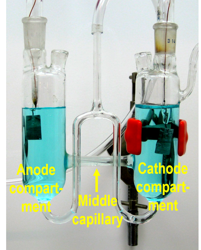
The disadvantage of the Hittorf method is that the duration of an experiment cannot be very long in order to prevent a concentration gradient from forming in the capillary connecting the compartments. During a brief experiment only rather small changes in concentrations occur, meaning the chemical analysis may be inaccurate. Current cannot be increased to an unlimited extent either because it would dissipate in the cell as heat.
In the method of a moving boundary, a vertical capillary is equipped with a cathode on the top and an anode on the bottom. Two solutions with a common ion (M+X– and N+X–) are poured into the capillary, with the denser solution on the bottom. In order to keep the boundary between the solutions sharp, the mobility of M+ must be higher than that of N+. The boundary resides initially at position A (see Figure 3.7). The system is electrolyzed with the charge \( Q=I\Delta t \), causing M+ to move upwards towards the cathode. The amount of M+ transferred is (t+Q)/(z+F) mol; the boundary is now at a new position B. The amount of M+ removed from the interval A-B is \( c_{MX}A\Delta x \) (A is the area of the cross section of the capillary and \( \Delta x \) the distance A-B). Equating these two expressions we find that
| \( t_+=\displaystyle\frac{z_+c_{MX}\Delta xAF}{I\Delta t} \) | (3.49) |
|---|
The ingenuity of the method is that the boundary remains sharp and diffusion does not blur it. The lower and denser solution usually contains an indicator so the boundary can be observed with the naked eye.
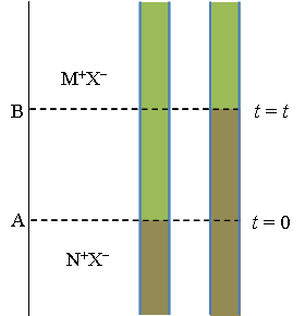
The velocity of an ion is given by Equation (3.5): vi = uiE. Since the conductivity of the lower solution, κ, is lower than in the upper solution the electric field E ~ i/κ is stronger in the lower solution. If M+ diffuses into the lower solution the stronger electric field accelerates it back into the upper solution, separating it from N+ that has lower mobility than M+. Accordingly, if N+ diffuses into the upper solution it experiences a lower electric field that decelerates it and it lags behind M+, bringing it back to the lower solution. However, if the conductivity of the lower solution is higher than in the upper solution the boundary does not remain sharp. A more detailed explanation is given in, I.N. Levine Physical Chemistry, McGraw-Hill, Tokio 1978, page 458-9 (removed from later editions!). |
|---|
Perhaps the most elegant method of determining a transport number is based on the electromotive force of a cell with transference, that is, its open circuit potential. For example, if two NaCl solutions at different concentrations are separated by a porous membrane or a frit that allows ions to diffuse across, Equation (3.46) gives the following for the diffusion potential (i = 0):
| \( \displaystyle \Delta\phi=\pm\frac{(2t_+-1)RT}{F}\text{ln}\left(\frac{c^\alpha}{c^\beta}\right) \) | (3.50) |
|---|
where \( \alpha \) and \( \beta \) refer to the two compartments. If the electrodes are reversible to Cl– anions, the Nernst equation contributes to the open circuit potential, making the total potential
| \( \displaystyle E=\pm\frac{2t_+RT}{z_+F}\text{ln}\left(\frac{a_{\text{Cl}}^\alpha}{a_{\text{Cl}}^\beta}\right) \) | (3.51) |
|---|
where concentrations are replaced by activities (see Equation (3.36)). The sign must be chosen depending on which concentration \( (c^{ \alpha} \text{ or } c^{\beta}) \) is higher. The measurement must be carried out with a voltage meter that has a very high input impedance to keep the current zero. The concentration difference between the compartments cannot be very large either. Cell potentials are revisited in Chapter 4.
3.5. Transport equation in a non-stationary state
The transport equations presented above apply only in steady state where the flux AJi (mol s-1) is not a function of the position but constant throughout the entire system; the flux density Ji (mol cm2 s-1) can vary depending on the cell geometry which is known as primary current distribution. In a non-stationary or transient state, solution concentrations vary as a function of location, and the flux is at its highest on the surface of the electrode. The non-stationary transport equation is reached calculating the divergence of the Nernst-Planck equation:
| \( \displaystyle\frac{\partial c_i}{\partial t}=-\nabla \cdot\vec{J}_i=D_i\nabla^2c_i+\frac{z_iF}{RT}D_i(\nabla c_i \cdot\nabla\phi+c_i\nabla^2\phi)-(c_i\nabla \cdot\vec{v}+\vec{v} \cdot\nabla c_i) \) | (3.52) |
|---|
It has been assumed above that the diffusion coefficient is independent of the concentration. In electroneutral systems, \( \nabla^2\phi=0 \) is known as the Laplace equation and its solutions as harmonic functions. Furthermore, in incompressible solutions \( \nabla \cdot\vec{v} =0 \) Therefore
| \( \displaystyle\frac{\partial c_i}{\partial t}=D_i\nabla^2c_i+\frac{z_iF}{RT}D_i\nabla c_i \cdot \nabla \phi-\vec{v}\nabla c_i \) | (3.53) |
|---|
In the supporting electrolyte case which is overwhelmingly the most common in electrochemistry, \( \nabla\phi \approx\frac{i}{\kappa}=0 \). Convection only concerns in hydrodynamic methods that will be discussed later. In the absence of convection, Equation (3.53) reduces to Fick’s second law:
\( \displaystyle\frac{\partial c_i}{\partial t}=D_i\nabla^2c_i \) |
(3.54) |
|---|
An electrochemical problem constitutes the solution of the above equation with the boundary condition (3.48) as well as other pertinent initial and boundary conditions, depending on the experimental method. These issues are addressed in Chapter 7.
You can now test your conceptual knowledge by taking Quiz Chapter 3.
4. Electrochemical cells
Electrochemical cell consists of an electrolyte solution, electrodes and an external circuit as defined in Chapter 1.1. Electrochemical cells can be divided into two main types depending on the spontaneity of the cell reaction. The cell reaction in galvanic cells is spontaneous, and chemical energy converts directly into electric energy. In other words, the \( \Delta \)G of the reaction is negative and therefore the cell potential according to equation (1.6) is positive. In electrolysis cells, electrical energy is converted to chemical energy. The cell reaction is hence forced towards the non-spontaneous direction and the \( \Delta \)G of an electrolysis cell is positive and cell potential negative.
Galvanic cells are used in everyday life as primary and secondary batteries and fuel cells. An unfortunate side effect of galvanic cell is electrochemical corrosion. Examples of electrolysis are, for example, charging of batteries, production of chlorine gas and sodium hydroxide from electrolysis of sodium chloride solution, and different electrochemical analysis methods. The most important analysis methods and the requirements for the electrochemical cell used in connection with them are introduced in Chapters 7 and 8.
We know from thermodynamics that the \( \Delta \)G of a reaction gives the maximum work available from a particular reaction. In practice, electrochemical cells are also more or less non-ideal, and efficiencies of 100% are not achieved. Deviations from ideal behavior stem from irreversible processes that take place when electric current flows, e.g. ohmic losses due to restricted electrolyte conductivity (Figure 4.1) and possible slowness of electrode reactions, which is seen as overpotentials (Chapter 6.3).
In this chapter, we discuss the description of electrochemical cells, the conventions associated with them and the formation of the cell potential. Applications of cells in equilibrium, potentiometry and pH-potential equilibrium diagrams are also briefly introduced. Finally, one of the most important cell structures for electrochemical analysis, the three-electrode set-up, is presented.
4.1. Electrochemical cell conventions
A number of conventions are needed in the presentation of electrochemical cells. First, reduction will always take place at the cathode and oxidation at the anode. Electrodes are called cathodes and anodes in both galvanic and electrolysis cells. Chapter 1 states that it is impossible to measure the potential of any particular electrode: one always measures or controls the potential difference between two electrodes, i.e. the cell potential. It is not appropriate to call electrodes cathodes and anodes in electrochemical analysis. The reaction of interest takes place at the working electrode and the other electrode in the system is called the counter electrode. The purpose of the counter electrode is to maintain the electroneutrality of the solution: the reaction occurring at the counter electrode is opposite the one taking place at the working electrode (oxidation or reduction). The potential difference between these two electrodes, the cell potential, is easily measurable. As seen in the simplified scheme in Figure 4.1, the cell potential is the sum of different potential differences. In Figure 4.1, the cell potential is composed of the electrode potentials due to a potential change as a result of an electric double layer (Chapter 5) close to the electrode surface. We will show later how this potential difference controls the faradic reactions taking place at the electrode. In addition, an ohmic iR drop affects the cell potential when current flows in the system. This iR drop is caused by the limited conductivity or the resistivity of the electrolyte solution, which is a function of the ionic strength, the dielectric constant of the solvent, and the distance between the electrodes. Only if the iR drop (or loss) can be assumed to be negligible can the measured cell potential be taken as the potential difference between the electrodes. Furthermore, different liquid junctions caused by the structure of the cell (Chapter 4.4.) can complicate the situation.
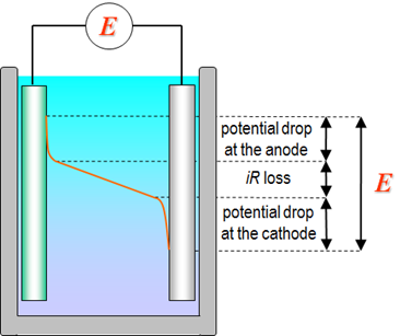
Figure 4.1. Potential profile in an electrochemical cell.
In electrochemical potentiometric methods, the aim is to accurately measure the potential of the working electrode. In electrochemical amperometric methods, the aim is to accurately control the potential of the working electrode and to measure the current. Because the experimental quantity to measure or control is the cell potential, it is clear that in order to accurately know the potential of working electrode, the potential of counter electrode needs to be constant and the iR drop contribution has to be negligible or known.
A counter electrode with a constant potential requires a half-cell where the exchange current density of the half-reaction is very large (Chapter 1.3.4) and the electrode is ideally unpolarizable. The solution components of the half-reaction need to be present in high concentration so the current passing through the electrode will not change the concentrations. An electrode like this is called a reference electrode. When current is flowing in the electrochemical cell, as is usually the case in electrochemical analysis, the use of two electrodes is not sufficient to accurately control the potential of working electrode. In these cases, so called three-electrode set-up is used (Chapter 4.7). 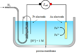
Figure 4.2. Galvanic cell with a standard hydrogen electrode as an anode and a gold electrode in Fe3+/Fe2+-solution as a cathode.
An example of a galvanic cell is presented in Figure 4.2. The standard hydrogen electrode is an anode; there is an agreed convention that it is always presented on the left-hand side of the scheme. The standard hydrogen electrode is a platinum black (very fine platinum powder) plated platinum disc. Hydrogen gas (at pressure of 1 bar) is passed over the disc in solution where the H+ ion concentration is 1 M. A gold electrode is immersed in a solution containing Fe3+ and Fe2+ ions. The acidic solution in the anode compartment and Fe3+/Fe2+ solution in the cathode compartment are separated from each other with a porous diaphragm. The purpose of the diaphragm is to prevent the direct mixing of the electrolyte solutions as this can lead to undesired side reactions and/or make the theoretical treatment of the cell difficult. Ions will pass through the diaphragm and hence current flows. The connection between the two solutions can also be achieved by using a salt bridge (Chapter 4.4.1).
A cell diagram shows the parts of a (galvanic) cell in a concise manner. The different phases in the cell are written from left to right. A boundary between two phases is represented with | and a salt bridge (or any other liquid junction with a small junction potential) with ||. The cell diagram for the cell in Figure 4.2 is:
Cu | Pt | H+, H2 || Fe3+, Fe2+ | Au | Cu
The copper phases on both ends are the conductors, which connect the cell to the potentiometer.
The electrochemical reactions that take place in the cell in Figure 4.2 are:
| at the cathode: Fe3++ e– \(\ce{ <=> }\) Fe2+ | (4.1) |
|---|
| at the anode: ½ H2 \(\ce{ <=> }\) H+ + e– | (4.2) |
|---|
Electric current is a property of a closed circuit. In this cell, electrons move from the hydrogen gas oxidising at the platinum anode through the external circuit to the cathode. At the cathode, electrons move back to the solution through the reduction of iron(III). In the solution, the current is carried by charged components, ions.
Combining reactions (4.1) and (4.2), the total cell reaction is:
| ½ H2 + Fe3+ \(\ce{ <=> }\) H+ + Fe2+ | (4.3) |
|---|
When considering electrochemical net cell reactions, it is advisable to keep in mind that the reaction equation represents a virtual reaction. The reaction species are not in direct contact through collisions in the solution, but the half-reactions take place heterogeneously on their corresponding electrodes. The equilibrium depicted by the reaction equation could only be realized if the electrons could move freely in the external circuit. If the cell is in equilibrium, the net current in the cell would be zero and the cell potential would be also zero (equation (1.6), at equilibrium \( \Delta \)G = 0). In practice, the external circuit holds a high-impedance potentiometer (or load if a galvanic cell is used as a source of voltage), which restricts the flow of current in the circuit. The use of a potentiometer in the circuit therefore results in a situation in which very little current flows in the system. This virtual equilibrium is discussed in the next chapters.
| The value of the cell potential in circumstances where no or very little current is flowing in the cell is an important measurable quantity. This quantity has several names: terminal voltage: maximum voltage available from a particular reaction EMF = electromotive force that moves the electrons equilibrium cell voltage: cell is at equilibrium reversible cell voltage: even a small change in the potential will cause current to flow null voltage/rest voltage: no current is flowing in the cell open circuit voltage: because movement of electrons in the external circuit is impeded, the situation is equivalent to the case of an open circuit |
|---|
Let us consider the measurement of the potential of the cell in Figure 4.2. According to an agreement, the potentiometer (voltmeter) is connected to a galvanic cell in such a manner that the potential is defined as the potential of the right-hand side electrode with reference to the left-hand side electrode *:
| Ecell = Eright – Eleft | (4.4) |
|---|
The electrode with reference to which the potential is measured and therefore the value of the potential is defined is the reference electrode. In the cell shown in Figure 4.2, the reference electrode is the standard hydrogen electrode on the left. The other electrode is the working electrode. It would often be useful to know the potential of a half-reaction. The measurement gives the total cell voltage, i.e. the difference between the half-cell potentials. In order to access the potential value for a half-reaction, another agreement is needed to divide the measured potential between the two half-reactions. This agreement and the measurement of standard potentials is presented in Chapter 4.3.
* In practice the voltmeter measures the galvani potential difference between the poles of the cell (Chapter 1.3.3). The poles of galvanic cells therefore need to be made of the same material.
4.2. Electrochemical cell potential at equilibrium
This chapter shows the derivation of cell potential for the cell in the previous chapter at virtual equilibrium. At equilibrium, the cell cannot be called a galvanic or electrolysis cell. Equilibrium is an important starting point for the examination of cell potentials, as the function of an electrochemical cell can be considered to approach thermodynamic equilibrium when the current flowing through the cell is close to zero. Potentiometric measurements are in practice very close to this situation. The cell potential (or cell voltage) is derived in two ways, first with Gibbs free energy change and equation (1.6) and second by considering the different equilibria at the phase boundaries through the concept of electrochemical potential.
The Gibbs free energy change for reaction (4.3) is:
| \( \displaystyle \Delta G=\Delta G^0+RT \ln \left[\frac{a_{\text{Fe}^{2+}}a_{\text{H}^{+}}}{a_{\text{Fe}^{3+}}(a_{\text{H}_2})^{1/2}}\right] \) | (4.5) |
|---|
and taking into account the relation between potential and Gibbs free energy change in equation (1.6) (n = 1, as seen from reaction equation) we get:
| \( \displaystyle E=E^0+\frac{RT}{F} \ln \left[\frac{a_{\text{Fe}^{3+}}(a_{\text{H}_2})^{1/2}}{a_{\text{Fe}^{2+}}a_{\text{H}^{+}}}\right] \) | (4.6) |
|---|
| In a general case, the Nernst equation for reaction aA + bB + cC.... \(\ce{ <=> }\) dD + eE + f F... is written as \( \displaystyle E=E^0-\frac{RT}{nF}\ln\left(\frac{a^d_Da^{e}_Ea^f_F...}{a^{a}_Aa^b_Ba^c_C...}\right) \) E0 can be obtained from tabulated values (Chapter 4.3.1) for half-reactions and n is the number of electrons exchanged in the total reaction. |
|---|
This is the Nernst equation for the potential of the cell in Figure 4.2. As seen from equation (4.6), the cell potential E corresponds to the standard cell potential E0, when the conditions are such that the activities inside the logarithm give the value 1.
Let us derive the potential for cell in Figure 4.2 via an equilibrium treatment. At equilibrium, all the phases in an electrochemical cell that are in direct contact with each other are in thermic, mechanical and chemical equilibrium. An equilibrium between two phases that are in contact does not require the presence of all components and species in all phases, or the chemical potential of each component to be the same in all of the phases. For example, the equilibrium between a metallic gold electrode and Fe3+ and Fe2+ ions in the solution does not contain gold in the solution phase or iron ions in the gold phase. The equilibrium takes place through electrons that are able to move freely across the phase boundaries.
It should be noted that the concept of an equilibrium in the treatment of electrochemical cells corresponds in a way to an impeded cell reaction. This equilibrium in an electrochemical cell can be achieved only if the external circuit is open or the impedance in the external circuit is so large that an electrochemical equilibrium is maintained at the phase boundaries despite a small current flowing through the system. It is also assumed that the system does not have irreversible phenomena such as corrosion, or the system does not exhibit temperature, pressure or concentration gradients.
The phases of the example cell are depicted as Greek symbols in the cell diagram below:
Cu | Pt | H+, H2 || Fe3+, Fe2+ | Au |Cu’
\( \alpha \) \( \beta \) \( \sigma \) \( \varepsilon \) \(\gamma \) \( \alpha \) .’
At equilibrium, the cell exhibits equilibria across the following phase boundaries: phase \( \alpha \) | phase \( \beta \), phase \( \beta \) | phase \( \sigma \), phase \( \sigma \) | phase \( \varepsilon \), phase \( \varepsilon \) | phase \( \gamma \) and phase \( \gamma \) | phase \( \alpha \)’. The chemical potential of an ion is an ill-defined quantity and hence the derivation uses the equality of the electrochemical potential (equation (2.7)) as the condition for equilibrium. The equilibria in the cell are as follows:
Phase \( \alpha \) | phase \( \beta \) i.e. the contact between copper wire and platinum electrode:
| \( \tilde\mu^{\beta}_{\text{e}^-}=\tilde\mu^{\alpha}_{\text{e}^-} \) | (4.7) |
|---|
Phase \( \beta \) | phase \( \sigma \) i.e. the equilibrium at platinum electrode (reaction equation 4.2):
| \( \tilde\mu^{\sigma}_{\text{H}^+}+\tilde\mu^{\beta}_{\text{e}^-}=\frac{1}{2}\tilde\mu^{\sigma}_{\text{H}_2} \) | (4.8) |
|---|
Phase \( \sigma \) | phase \( \varepsilon \), the interface between two liquid phases, in practice often a salt bridge. In this simple derivation, we will assume that the inner potential of the solution is the same in both sides of the interface. Some cases where this assumption is not done will be covered later on (junction potentials, chapter 4.4).
| \( \phi^{\sigma}= \phi^{\varepsilon} \) | (4.9) |
|---|
Phase \( \varepsilon \) | phase \( \gamma \) i.e. the equilibrium at the gold electrode (reaction equation 4.1)
| \( \tilde\mu^{\varepsilon}_{\text{Fe}^{3+}}+\tilde\mu^{\gamma}_{\text{e}^-}=\tilde\mu^{\varepsilon}_{\text{Fe}^{2+}} \) | (4.10) |
|---|
Phase \( \gamma \) | phase \( \alpha \)’ i.e. the contact between copper wire and gold electrode:
| \( \tilde\mu^{\gamma}_{\text{e}^-}=\tilde\mu^{\alpha}_{\text{e}^-} \) | (4.11) |
|---|
By using equation (2.7), these equilibrium conditions can be presented as:
| \( F\left(\phi^{\beta}-\phi^{\alpha}\right)=\mu_{\text{e}^-}^{\beta}-\mu_{\text{e}^-}^{\alpha} \) |
(4.12) |
|---|---|
| \( \displaystyle F\left(\phi^{\sigma}-\phi^{\beta}\right)=\left(\frac{1}{2}\mu^0_{\text{H}_2}-\mu_{\text{H}^+}^0-\mu_{\text{e}^-}^{\beta}\right)+RT\ln\left(\frac{(a_{\text{H}_2})^{1/2}}{a_{\text{H}^+}}\right) \) |
(4.13) |
| \( \displaystyle F\left(\phi^{\gamma}-\phi^{\varepsilon}\right)=\left(\mu^0_{\text{Fe}^{3+}}-\mu_{\text{Fe}^{2+}}^0+\mu_{\text{e}^-}^{\gamma}\right)+RT\ln\left(\frac{a_{\text{Fe}^{3+}}}{a_{\text{Fe}^{2+}}}\right) \) |
(4.14) |
| \( F\left(\phi^{\alpha '}-\phi^{\alpha\gamma}\right)=\mu_{\text{e}^-}^{\alpha'}-\mu_{\text{e}^-}^{\gamma} \) | (4.15) |
Combining equations (4.12)-(4.15) and taking into account (4.9) the cell potential i.e. the galvanic potential difference between the two copper wires is obtained as (note that the chemical potentials of the wires are equal because the phases are identical):
| \( F\left(\phi^{\alpha}-\phi^{\alpha'}\right)=\left(\mu^0_{\text{Fe}^{3+}}-\mu_{\text{Fe}^{2+}}^0+ \frac{1}{2}\mu^0_{\text{H}_2}-\mu_{\text{H}^+}^0\right)+RT\ln\left(\frac{a_{\text{Fe}^{3+}}(a_{\text{H}_2})^{1/2}}{a_{\text{Fe}^{2+}}a_{\text{H}^{+}}}\right) \) |
(4.16) |
| \( \displaystyle E_{\text{cell}}=E^0+\frac{RT}{F} \ln \left[\frac{a_{\text{Fe}^{3+}}(a_{\text{H}_2})^{1/2}}{a_{\text{Fe}^{2+}}a_{\text{H}^{+}}}\right] \) | (4.17) |
|---|
which naturally corresponds to equation (4.5) that was obtained earlier. Let us consider equation (4.17) further, keeping in mind the relationship between the Gibbs free energy change and the potential (equation (1.6)). If the virtual total cell reaction (4.3) of our cell is exergonic (\( \Delta \)G < 0), hydrogen gas can, as described in the reaction equation, reduce Fe3+. This reaction produces work, and if the potentiometer in Figure 4.2 is replaced by a load, the work of the reaction can be utilized. This work corresponds to the transfer of electrons from the gold electrode to the platinum electrode (in solution), and in an ideal case the value of this work is –FEcell.
4.3. Standard potential
Quantity E0 in equations (4.5) and (4.17) is the standard value for cell potential. Thermodynamics defines certain standard conditions in order to enable reliable comparison of quantities and preparation of tables. In the example cell, the standard cell potential can be divided in two parts. These two parts are thought to be the contributions of the potential that each electrode reaction produces:
| \( E^0=E^0_{\text{Fe}^{3+}/\text{Fe}^{2+}}-E^0_{\text{H}^{+}/\text{H}_{2}} \) |
(4.18) |
|---|
where
| \( -FE^0_{\text{H}^{+}/\text{H}_{2}}=\mu^0_{\text{H}^+}-\frac{1}{2}\mu^0_{\text{H}_2} \) | corresponding to the half-cell Pt | H+,H2 |
|---|---|
| \( -FE^0_{\text{Fe}^{3+}/\text{Fe}^{2+}}=\mu^0_{\text{Fe}^{2+}}-\mu^0_{\text{Fe}^{3+}} \) | corresponding to the half-cell Fe3+,Fe2+ | Au |
Combining the half-cells gives the E0 of the example cell:
| \( \displaystyle E^0=\frac{\mu^0_{\text{Fe}^{3+}}-\mu^0_{\text{Fe}^{2+}}-\mu^0_{\text{H}^{+}}+\mu^0_{\text{H}_{2}}}{F}=\frac{-\Delta G^0}{nF} \) | (4.19) |
|---|
The standard potential of the cell gives the work needed to transfer one electron between the gold electrode and the redox couple (Fe3+/Fe2+) in the solution, on a potential scale that is defined by the hydrogen electrode on the left side of the cell in standard conditions. Standard potentials of different half-cells are tabulated and combining these gives the standard cell potential of galvanic cells. The tabulated values of E0 also enable the estimation of spontaneity of different reactions. As seen from (4.19), the larger the value of standard reduction potential, the stronger the driving force for a particular reaction (as the more negative the value of Gibbs free energy change). This allows conclusions concerning half-reactions, e.g. choosing which half-reaction in galvanic cell is oxidation and which is reduction.
One has to keep in mind that the standard potential for a half-cell is not the same as the “absolute” electrode potential i.e. the galvani potential difference. The standard electrode potential for the half-cell Pt | H+,H2 based on equation (4.13) is
|
(4.20) |
|---|
whereas \( E^0_{\text{H}^+/\text{H}_2} \) is obtained from (4.17)
| \( \displaystyle E^0_{\text{H}^+/\text{H}_2}=\frac{\frac{1}{2}\mu^0_{\text{H}_{2}}-\mu^0_{\text{H}^{+}}}{F} \) | (4.21) |
|---|
\( (\phi^{\sigma}-\phi^{\beta}) \) and hence also \( E^0_{\text{H}^+/\text{H}_2} \) cannot either be measured. An auxiliary agreement is therefore needed to enable the potentials of the half-cells to be defined. According to the standard hydrogen electrode convention of IUPAC[1], the half-cell potential of the standard hydrogen electrode (left side of Figure 4.2.) at all temperatures is zero:
\( E^0_{\text{H}^{+}/\text{H}_{2}} \equiv0\text{V} \) |
(4.22) |
|---|
Example 1: Why is FeCl3 used to dissolve copper in the manufacture of circuit boards? Justify your answer with the standard reduction potentials below.
\( E^0_{{\text{Fe}^{3+}}/{\text{Fe}^{2+}}}=0.77\text{V} \) \( E^0_{{\text{Cu}^{2+}}/{\text{Cu}^{+}}}=0.34\text{V} \)
Tabulated values of reduction potentials correspond to the standard potentials of the following reactions: Fe3+ + e– → Fe2+ E0 = 0.77 V Cu2+ + 2e– → Cu E0 = 0.34 V
Let us combine these into a reaction where Fe(III) ions dissolve metallic copper: 2Fe3+ + 2e– → 2Fe2+ E0 = 0.77 V Cu → Cu2+ + 2e– E0 = –0.34 V ____________________________________________________________________________ 2Fe3+ + Cu →2Fe2+ + Cu2+ E0total = 0.43 V
When combining half-reactions, one has to remember to balance the number of transferring electrons by multiplying the half-reactions with appropriate numbers. Even if the half-reaction is multiplied by a number (like here the reaction of iron by 2), the corresponding standard potential is not multiplied as the potential is an intensive quantity. Both DG0 and n are extensive quantities, so the ratio of them is an intensive quantity (not dependent on the amount of substance). The tabulated potential values are for reduction, and since the reaction of copper is reversed for oxidation, the sign of the corresponding potential is also reversed. The standard cell potential for the total cell reaction is obtained as the sum of the half-reaction potentials (potential is a state function). The Gibbs free energy change for the reaction (in standard conditions) is obtained as:
The reaction is spontaneous as the Gibbs free energy change is negative. A Fe(III) ion in the solution will dissolve (oxidize) metallic copper. |
|---|
4.3.1 Standard potential values
The standard potential E0 of a cell can be obtained in four ways:
· from the standard Gibbs free energy change of the virtual total cell reaction
· from the tabulated standard reduction potentials of the half-reactions
· from the equilibrium constant K of the virtual total cell reaction
· extrapolating from experimental results
Example 2: There are two approaches in the literature to calculate the E0 of a (galvanic) cell from the tabulated values of the E0 of half-reactions. Example 1 presents the approach where one of the two reduction reactions is reversed into an oxidation reaction. As the half-reaction is reversed, the sign of the reduction potential is changed. A virtual net cell reaction is obtained by adding the reduction and oxidation reactions, and because the potential is a state function, the potential of the sum reaction (the net cell reaction) is obtained as the sum of the reduction and oxidation potentials.
E.g. Daniel cell: Zn | 1.0 M Zn2+ || 1.0 M Cu2+ | Cu
Reduction potentials from a table: Zn2+ + 2e– \(\ce{ -> }\) Zn E0 = –0.76 V Cu2+ + 2e– \(\ce{ -> }\) Cu E0 = 0.34 V
The reaction of zinc is reversed to an oxidation reaction and the sign of the corresponding potential is changed. The virtual net cell reaction and its standard potential E0 is obtained as a sum: Zn \(\ce{ -> }\) Zn2+ + 2e– E0 = 0.76 V Cu2+ + 2e– \(\ce{ -> }\) Cu E0 = 0.34 V _____________________________________________________________ Zn + Cu2+ \(\ce{ -> }\) Zn2+ + Cu E0 = 0.76 V+ 0.34 V = 1.1 V
According to the second approach, the cell potential is calculated from equation (4.4) as Ecell = Eright – Eleft. In a galvanic cell, the reaction on the right is reduction and the reaction on the left is oxidation. Therefore, for the Daniel cell:
E0 = 0.34V – (–0.76 V) = 1.1 V
It is necessary to know which of the half-reactions is reduction and which is oxidation. The rule of thumb is that the reaction that has the lower reduction potential is converted to oxidation.
|
|---|
Quite often one needs to measure the standard potential of a half-reaction. As the standard hydrogen electrode defines the zero of the potential scale, the desired half-cell can be determined by constructing a cell that has this as the other electrode. A silver-silver chloride electrode is a typical reference electrode, which can be prepared by electrolyzing a silver wire in a solution containing chloride, thus forming a solid layer of silver chloride at the surface of the silver wire. In order to find the standard potential of the silver-silver chloride electrode, the following cell can be constructed in standard conditions:
| Cu | Pt | H2, HCl | AgCl | Ag | Cu’ | (4.23) |
|---|
Half-reactions are now written in terms of reduction, like the tabulated values:
| Ag+ + e– \(\ce{ <=> }\) Ag | (4.24a) |
|---|---|
| H+ + e– \(\ce{ <=> }\) ½ H2 | (4.24b) |
The cell potential is obtained from the corresponding Nernst equations and equation (4.4):
| \( \displaystyle E=\left[E^0_{\text{Ag}^+/\text{Ag}}+\frac{RT}{F}\ln\left(\frac{a_{\text{Ag}^+}}{a_{\text{Ag}}}\right)\right]-\left[E^0_{\text{H}^+/\text{H}_2}+\frac{RT}{F}\ln\left(\frac{a_{\text{H}^+}}{(a_{\text{H}_2})^{1/2}}\right)\right] \) | (4.25) |
|---|
Let us assume that the silver electrode is made of pure silver and, therefore, its activity is one. In addition, equation (4.22) defines that the standard reduction potential of H+/H2 is zero, and equation (4.25) becomes
| \(\displaystyle E=E^0_{\text{Ag}^+/\text{Ag}}+\frac{RT}{F}\ln\left(\frac{a_{\text{Ag}^+}(a_{\text{H}_2})^{1/2}}{a_{\text{H}^+}}\right) \) | (4.26) |
|---|
At the surface of the right-hand side electrode of cell (4.23), the equilibrium is achieved with chloride ions. Silver chloride is a sparingly soluble salt, and the chloride ion activity can be taken into equation (4.26) with the help of the solubility product, Ks = 1.77×10⁻¹⁰. It is the equilibrium constant of the reaction:
| AgCl \(\ce{ <=> }\) Ag++ Cl– | (4.27) |
|---|
Hence, because AgCl is a pure, solid compound with the unit activity,
| \( \displaystyle K_s=\frac{a_{\text{Ag}^+}a_{\text{Cl}^-}}{a_{\text{AgCl}}}=a_{\text{Ag}^+}a_{\text{Cl}^-}\cong\frac{c_{\text{Ag}^+}c_{\text{Cl}^-}}{(c^0)^2} \) | (4.28) |
|---|
Combining (4.26) and (4.28), and replacing the activity of the gas with its fugacity ratio at the reference pressure (according to the definition of activity) gives:
| \( \displaystyle E= E^0_{\text{Ag}^+/\text{Ag}}+\frac{RT}{F}\ln\left(\frac{K_s(a_{\text{H}_2})^{1/2}}{a_{\text{H}^+}a_{\text{Cl}^-}}\right)= E^0_{\text{Ag}^+/\text{Ag}}+\frac{RT}{F}\ln K_s+\frac{RT}{2F}\ln\left(\frac{f_{\text{H}_2}}{p^0}\right)-\frac{RT}{F}\ln(a_{\text{H}^+}a_{\text{Cl}^-}) \) | (4.29) |
|---|
Constant terms in (4.29) form the standard reduction potential of the Ag/AgCl electrode. The value of this standard potential can be calculated from the standard reduction potential of silver and the solubility product of AgCl:
| \( \displaystyle E^0_{\text{AgCl/Ag}}=E^0_{\text{Ag}^+/\text{Ag}}+\frac{RT}{F}\ln K_s=0.799\text{ V}-0.577\text{ V}=0.222\text{ V} \) | (4.30) |
|---|
If the fugacity of the hydrogen gas is kept constant at 1 bar (standard conditions), the third term on the right-hand side of equation (4.29) is zero. In this case, the cell potential of (4.22) is a direct function of HCl concentration. Measuring the cell potential as a function of the concentration and extrapolating to infinite dilution, where the activity coefficient can be estimated with unity, the experimental value for standard reduction potential is obtained:
| \( \displaystyle E^0_{\text{AgCl/Ag}}=\lim\left(E+\frac{RT}{F}\ln(c_{\text{H}^+}c_{\text{Cl}^-})\right)_{c_{\text{HCl}}\rightarrow0} \) | (4.31) |
|---|
A hydrogen electrode with bubbled gas supply is not the most practical choice. As a matter of fact, the Ag/AgCl electrode in the previous example is currently the most popular reference electrode. Another popular choice is the calomel electrode, although it contains mercury salts (e.g. Hg2Cl2). Figure 4.3. presents the measurement of cell potential with Ag/AgCl electrode as the reference electrode instead of the hydrogen electrode.
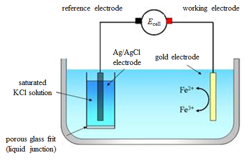
Figure 4.3. A galvanic cell for the determination of the standard potentials using the Ag/AgCl reference electrode.
This cell can be represented by the following cell diagram:
| Cu | Ag | AgCl | KCl(sat.) || Fe3+, Fe2+ | Au |Cu’ | (4.32) |
|---|
The cell potential is
| \( \displaystyle E=\left[E^0_{\text{Fe}^{3+}/\text{Fe}^{2+}}+\frac{RT}{F}\ln\left(\frac{a_{\text{Fe}^{3+}}}{a_{\text{Fe}^{2+}}}\right)\right]-\left[E^0_{\text{AgCl/Ag}}-\frac{RT}{F}\ln(a_{\text{Cl}^-})\right] \) | (4.33) |
|---|
Combining the constant terms in equation (4.33) (activity of Cl− is constant because the solution is saturated) gives
| \( \displaystyle E=\left[E^{\text{0,AgCl/Ag}}_{\text{Fe}^{3+}/\text{Fe}^{2+}}+\frac{RT}{F}\ln\left(\frac{a_{\text{Fe}^{3+}}}{a_{\text{Fe}^{2+}}}\right)\right] \) | (4.34) |
|---|
where \( E^{\text{0,AgCl/Ag}}_{\text{Fe}^{3+}/\text{Fe}^{2+}} \) is the standard reduction potential for the Fe(II)/Fe(III) redox pair on the scale of the Ag/AgCl reference electrode with the saturated KCl solution. As with the measurement with the standard hydrogen electrode, cell potentials are measured at different iron ion concentrations and the results extrapolated to infinite dilution to access the standard potential at the working electrode.
Standard potentials can also be determined with other experimental methods. Chapter 7 describes the use of cyclic voltammetry to determine the standard potential of a half-reaction. In addition, standard potentials can be resolved by combining electrochemical methods with spectroscopic methods.
4.3.2 Standard potentials on absolute scale
Electrochemical methods are used to measure the ionization potentials of conducting polymers or to determine the HOMO and LUMO orbital energies of organic molecules. The values typically obtained with cyclic voltammetry and the Ag/AgCl reference electrode need to be converted into what is known as the absolute scale and presented in electron volts (eV). The reference point of the absolute scale is a vacuum and the scale is also called the ‘vacuum scale’. The link between the standard hydrogen scale and the absolute scale is derived next. A more detailed account can be found in the literature[2].
Let us consider a case in which the standard potential of a redox couple in a solution is measured with the standard hydrogen electrode as the reference electrode. Let us assume that the electrostatic effect due to the surface potential of the electrolyte can be omitted (c s =0).
| \( \displaystyle E^{0, \text{abs}}_{\text{red/ox}}=\phi^{\text{metal}}-\phi^{\text{solution}}-\frac{\mu^{\text{M}}_{\text{e}}}{F}+\chi^S=\frac{\left(\alpha^0_{\text{H}^+}-\frac{1}{2}\mu^0_{\text{H}_2}\right)}{F} \) | (4.35) |
|---|
\( E^{0, \text{abs}}_{\text{red/ox}} \) is the standard reduction potential of the redox couple on the absolute scale, \( \alpha^0_{\text{H}^+} \) is the true standard chemical potential of the proton in the solution (i.e. the electrochemical potential in a non-charged environment) and \( \mu^0_{\text{H}_2} \) is the standard chemical potential of the gaseous hydrogen molecule. In order to find the value of equation (4.35), it is very important to use the same reference point for all the quantities in the equation, the reference point being a vacuum. The standard chemical potential for a gaseous hydrogen molecule can be estimated from the ionization energy of the hydrogen atom and the covalent bond energy of the hydrogen molecule:
H+(g) + e−(g) \(\ce{ <=> }\) H(g) \( \Delta \)G0 = −13.613 eV
H(g) \(\ce{ <=> }\) ½ H2(g) \( \Delta \)G0 = −2.107 eV
The real standard chemical potential of the proton in an aqueous solution is
H+(g) \(\ce{ <=> }\) H+(aq) \( \alpha^0_{\text{H}^+} \) −11.276 eV
The standard potential of the hydrogen electrode on the absolute scale in Volts is:
| \( \displaystyle E^{0,\text{abs}}_{\text{H}^+/\text{H}_2}\cong\left[-11.276-(-13.613-2.107)\right]=4.44\text{ V} \) | (4.36) |
|---|
The potential values measured with reference to the standard hydrogen electrode (SHE) can be converted to the absolute scale with
| \( E^{0, \text{abs}}_{\text{Red/Ox}}\cong E^{0, \text{SHE}}_{\text{Red/Ox}}+4.44\text{ V} \) | (4.37) |
|---|
If the potential values have been determined using another reference electrode, the potential values are first converted to the SHE scale and then to the absolute scale. Potential values for different reference electrodes can be found in the literature (taking into account the different concentrations of the inner solutions of the electrodes) at different temperatures.
Example 3: Energy diagram to be drawn for the conducting polymer polyhexylthiphene (PHT) based on the following information: the oxidation potential from cyclic voltammetry for the polymer E’ox (vs. Ag/AgCl) was 0.40 V and the band gap Eg from spectroscopic measurements was 2.0 eV.
Solution: An energy diagram presents the HOMO (highest occupied molecular orbital) and the LUMO (lowest un-occupied molecular orbital) of a molecule. In solid substances, these are called the valence band and the conduction band, respectively. These can be estimated from the first oxidation potential of a semiconductor (HOMO, valence band) and the first reduction potential (LUMO, conduction band). The ionization energy (IE) of PHT, i.e. the energy of HOMO is obtained from the oxidation potential that is measured with cyclic voltammetry. The measurement used Ag/AgCl as the reference electrode so the value of the potential has to be converted to the absolute scale. The standard potential of Ag/AgCl electrode (25 °C, saturated KCl solution) is +0.199 V on the standard hydrogen scale, and the oxidation potential on the SHE scale is:
E’ox (vs. SHE) = E’ox (vs. Ag/AgCl) + 0.199V = 0.40 V + 0.199 V = 0.60 V,
and converted further to the absolute scale according to equation (4.37):
Eox (abs) = 0.60 V + 4.44 V = 5.04 V,
and to electron volts IE =e Eox (abs) = 5.04 eV
The energy diagram can now be drawn: |
|---|
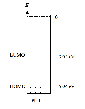
[1] IUPAC = International Union of Pure and Applied Chemistry
[2] H.H. Girault, Analytical and Physical Electrochemistry, EPFL Press, 2004.
4.4. Cells with transference
The assumption up until now in this chapter has been that there is a heterogeneous equilibrium on each phase boundary. A cell reaction will proceed reversibly in both directions if the equilibrium is disturbed slightly. If liquid junctions are present in the cell, they cause a particular, non-measurable potential loss in the cell. A typical case where this kind of potential losses is found is a cell in which two solutions with different compositions are in direct contact with each other. Concentration gradients will force the different species in the system to transfer from one phase to another. If these species involve ions, a diffusion potential is formed between the solution phases. If a diaphragm or a membrane separates the phases, ionic transport creates a membrane potential between the phases. In practice, the cells in Figures 4.2 and 4.3 contain liquid junctions. In chapters 4.3-4.4 this potential loss was assumed to be insignificant and, therefore, was not taken into account. In those exemplary cells, the liquid junctions would form over the diaphragm in Figure 4.2 and the porous diaphragm of the Ag/AgCl electrode structure in Figure 4.3.
4.4.1 Liquid junctions
A liquid junction potential between two solutions is formed when:
· solutions are in direct contact
· solutions contain different ions at different concentrations
· ions have different mobilities
A very common example of a liquid junction is the calomel (or the Ag/AgCl) electrode. It is used as a ‘universal’ reference electrode as it can be immersed in almost any aqueous solution. In many cases, no reference electrode is truly fully reversible with respect to the ion/s present in the solution. Furthermore, reference electrodes are often either also prone to interference by other ions or do not work reliably in concentrated solutions – a fact that often limits the use of ion-selective electrodes.

![]()
When a calomel electrode is immersed in, for example, a phosphate buffer solution at pH 7, a liquid junction is formed across the glass frit of the electrode. Inside the electrode there are K+ and Cl− ions, whilst H+, H2PO4− and HPO42 − ions are present in the measurement solution. In the frit, there is a mixture of all these ions and their concentrations will vary as a function of position in an unknown manner. In principle, the solution of the liquid junction potential follows equation (3.49) there is no electric current present, i.e. i = 0. Since the transport numbers are functions of the ionic concentrations, there is no exact solution of the problem in a multi-ionic system as the exact concentration profiles are unknown. Assuming that all the ions have a similar concentration profile across the glass frit, namely
| \( \displaystyle c_i(x)=c_i^{in}+(c_i^{out}-c_i^{in})·g(x) \) |
(4.38a) |
|---|
where g(x) is an undetermined function that has the property g(0) = 0 and g(h) = 1 (h is the frit thickness), the integration of equation (3.49) leads to the following useful form:
| \(\displaystyle \Delta \phi= \phi^{out}- \phi^{in}=- \frac{RT}{F} \frac{\sum\limits_{i}z_iD_i(c_i^{out}-c_i^{in})}{\sum\limits_{j}z_j^2D_j(c(j^{out}-c_j^{in})}ln \frac{\sum\limits_{k}z_k^2D_kc_k^{out}}{\sum\limits_{l}z_l^2d_lc_l^{in}} \) |
(4.38b) |
|---|
Equation (4.38b) is known as the Henderson equation. Let us assume that the inner solution is 1 M KCl and the outer (measurement) solution is a 0.1 M phosphate buffer at pH 7 with the following ionic concentration (in mol/dm3): H+, 10−7; Na+, 0.158; H2PO4− 0.042; HPO42 − 0.058. The contribution of H+ can be omitted, as its concentration is orders of magnitude lower than that of the other ions. By using the diffusion coefficient values given in Appendix 2 and presuming that the diffusion coefficients of the phosphate species are approximately 10−5 cm2/s, equation (4.38b) gives \Delta f ≈ −2 mV. This calculation shows that junction potentials are very small and are, therefore, usually omitted from the cell potential. Although, there are more elaborate treatises of the junction potential in essence they do not change the overall picture, except in some special cases.
4.4.2 Concentration cells
A concentration cell has identical electrodes and electrode reactions. In principle, if two identical electrodes are immersed in the same solution, the cell potential will be zero (equation 4.4). However, if the electrodes are immersed in solutions which differ only in their concentrations, a cell potential will form. The solutions have to include an ion with respect to which the electrode is reversible.
Let us consider a cell that has two identical Ag/AgCl electrodes immersed in KCl solutions of different concentrations:
| Ag | AgCl | KCl(I).|.(series of solutions).|. KCl(II) | AgCl’ | Ag’ | (4.39) |
|---|
The cell potential is formed as the sum of the galvanic potential differences between the phases:
| \( E_\text{cell}=(\phi_\text{Ag/AgCl'}-\phi_\text{KCl(II)})+(\phi_\text{KCl(II)}-\phi_\text{KCl(I)})+(\phi_\text{KCl(I)}-\phi_\text{Ag/AgCl}) \) | (4.40) |
|---|
In equation (4.40), (\( \phi_\text{Ag/AgCl'}-\phi_\text{KCl(II)} \)) and (\( \phi_\text{KCl(I)}-\phi_\text{Ag/AgCl} \)) are the electrode potentials and (\( \phi_\text{KCl(II)}-\phi_\text{KCl(I)} \)) is the potential difference between solution phases I and II. The electrodes are reversible with respect to the chloride ion. Electrochemical equilibrium gives:
| \( \mu_{\text{Cl}^-}^\text{I}-F\phi_\text{KCl(I)}=\mu_{\text{Cl}^-}^\text{Ag/AgCl}-F\phi_\text{Ag/AgCl} \) |
(4.41) |
|---|---|
| \( \mu_{\text{Cl}^-}^\text{II}-F\phi_\text{KCl(II)}=\mu_{\text{Cl}^-}^\text{Ag/AgCl'}-F\phi_\text{Ag/AgCl'} \) |
(4.42) |
Taking into account the similarity of the electrodes, which makes the chemical potential of chloride ion equal in both electrodes, gives:
| \( (\phi_\text{Ag/AgCl'}-\phi_\text{Ag/AgCl})=(\phi_\text{KCl(II)}-\phi_\text{KCl(I)})- \frac{1}{F}(\mu_{\text{Cl}^-}^\text{II}-\mu_{\text{Cl}^-}^\text{I}) \) | (4.43) |
|---|
Potential difference between KCl solutions of different concentrations is calculated using the equation of diffusion potential, Equation (3.49). This gives in a one-dimensional case, which when added up over all the ions in the solution is:
| \(\displaystyle (\phi_\text{KCl(II)}-\phi_\text{KCl(I)})= \int_\text{I}^\text{II}{d\phi}=- \frac{1}{F} \int_\text{I}^\text{II} \sum\limits_k \frac{t_k}{z_k}d\mu_k \) | (4.44) |
|---|
The cell potential is obtained by inserting (4.44) into (4.43):
| \(\displaystyle E_\text{cell}=(\phi_\text{Ag/AgCl'}-\phi_\text{Ag/AgCl})=-\frac{1}{F} \left[(\mu_{\text{Cl}^-}^{\text{II}}-\mu_{\text{Cl}^-}^{\text{I}})+ \int_\text{I}^\text{II}{\sum\limits_k} \frac{t_k}{z_k}d\mu_k \right] \) | (4.45) |
|---|
Because transport numbers are constants in a binary solution, equation (4.45) can be integrated to give
| \( \displaystyle E_\text{cell}=- \frac{2t_{\text{K}^+}RT}{F}ln \left( \frac{a_{\text{Cl}^-}^\text{II}}{a_{\text{Cl}^-}^\text{I}}\right) \) | (4.46) |
|---|
where the relation \( t_{\text{K}^+}+t_{\text{Cl}^-}=1 \) and equation (2.20) have been applied.
4.5. Pourbaix diagram
As is clear by now, standard potentials can be used to deduce the direction of redox reactions. Corrosion of metals often involves acid-base reactions coupled with redox reactions. The thermodynamic treatment of corrosion often involves the dependence of reactions on the equilibrium potential and pH. This is presented in a graphic form known as the Pourbaix diagram. It is an isothermic equilibrium diagram, usually presented at 25 °C. The vertical axis is the thermodynamic equilibrium potential on the standard hydrogen electrode scale and the horizontal axis is the pH of the solution in contact with the metal phase. Ionic concentrations have usually been fixed to 10-6 M. Figure 4.4 presents the Pourbaix diagram of iron. The thermodynamically stable species is marked on each zone of the diagram. The lines are defined by electrochemical or acid-base equilibria of the species present. The upper dashed line is the equilibrium potential of the oxygen electrode and the lower dashed line that of the hydrogen electrode, i.e. they represent the potential limits at which the oxygen and hydrogen evolution reactions begin to occur.
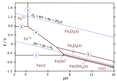
Figure 4.4. Pourbaix diagram of iron. T = 25ºC and ionic concentrations 10–3 M. Source: https://chem.libretexts.org/
The horizontal lines describe pH independent equilibria. For example, line 1 is the equilibrium Fe2+ + 2 e– \(\rightleftharpoons \) Fe which is dependent on potential according to the Nernst equation
| \( \displaystyle E=E_{\text{Fe}^{2+}/\text{Fe}}^0+ \frac{RT}{2F} ln\left(c_{\text{Fe}^{2+}}\right) \) | (4.47) |
|---|
Inserting values into the Nernst equation gives E = –0.53 V, which is the expression corresponding to line 1.
Vertical lines represent pH-dependent equilibria with no electron transfer (i.e. they are independent of potential). For example, line 3 represents equilibrium
2 Fe3+ + 3 H2O \( \rightleftharpoons \) Fe2O3(s) + 6 H+
with equilibrium constant
| \( \displaystyle K= \frac{(c_{\text{H}^+})^6}{(c_{\text{Fe}^{3+}})^2} \) | (4.48) |
|---|
and the expression for line 3 is pH = 0.1 because logK = 0.90 and [Fe3+] = 10-3 M.
All sloped lines in the diagram represent equilibria, which are dependent on both potential and pH. For example, line 4 represents equilibrium
Fe2O3(s) + 6 H++ 2e– \( \rightleftharpoons \) 2 Fe2+ + 3 H2O
The Nernst equation for this equilibrium is
| \( \displaystyle E=E_{\text{Fe}_2\text{O}_3/\text{Fe}^{2+}}^0+ \frac{RT}{2F}ln \frac{(c_{\text{H}^+})^6}{(c_{\text{Fe}^{3+}})^2} \) | (4.49) |
|---|
The expression for line 4 is E/V = 0.91 − 0.18·pH.
The Pourbaix diagram includes the equilibrium potentials of hydrogen and oxygen electrodes as dashed lines. The difference between these lines is 1.23 V, which is the thermodynamic dissociation potential of water. Above the oxygen electrode line, water is spontaneously dissociating and oxygen is evolving, below the hydrogen electrode line water is dissociating and hydrogen gas is evolving. Most corrosion reactions take place in the domain between these lines where water is stable.
Assuming that all solid oxides or hydroxides will form a passivating film on the metal surface, the Pourbaix diagram gives the zones where metal should be immune, active (corroding) or passive (not corroding or corroding only very slightly).
A Pourbaix diagram of a metal shows the conditions for the metal to remain passive or immune to the corrosive effects of the environment. The information from the diagram has to be used with caution as it is based purely on thermodynamics. The most important restrictions are
· The assumption of equilibrium between the metal, its ions, and its ions and different solid corrosion products. In practice, equilibrium may not be reached but the kinetics of the corrosion reactions dictates the reaction and the structure of the products.
· The pH-value in the diagram is a surface value. In practice, pH can vary locally and is usually lower on the anode surfaces and higher on the cathode surfaces compared to the value measured from the bulk solution.
· Thermodynamics does not tell the structure of the solid corrosion products, or how well they actually protect the metal from corrosion. Passive zones in the diagram need to be confirmed experimentally.
· The Pourbaix diagram does not provide any information on the rate of corrosion, which is dependent on the kinetics of the corrosion reaction
4.6. Potentiometry
Potentiometric methods provide an accurate means to measure the cell potential. In an elementary measurement, the Nernst equation is applied to find the relation between the concentration and the measured cell potential. Potentiometric measurements can be used to determine, for example, standard potentials, concentrations of electroactive species, mean activity coefficients of electrolytes, acid and base constants, stability constants of complexes, and equilibrium constants of redox reactions. An example of determining the standard potential of the Ag/AgCl electrode was presented in chapter 4.3.1.
The best-known example of a widely used potentiometric measurement is the determination of pH. A pH meter typically uses an Ag/AgCl as the reference electrode and what is known as the glass electrode as the working (or indicator) electrode. The glass electrode is an example of ion-selective electrodes, which are used in various chemical environments to determine concentrations. The heart of an ion-selective electrode is a semipermeable membrane; the potential difference across the membrane depends only on the concentration of the species of interest.
The tip of the glass electrode is made of glass, and the inside of the electrode holds HCl solution at the constant concentration. The electrodes (the reference and indicator electrodes are usually made into one structure) are immersed in the studied solution. The potential change across the glass membrane is dependent on the activity difference between protons in the inner liquid and the studied solution. The Ag/AgCl reference electrode detects this potential. According to the Nernst equation:
| \( \displaystyle E=\text{constant}-\frac{RT}{F}\ln\left(\frac{a_{\text{inner}}}{a_{\text{solution}}}\right) \) | (4.50) |
|---|
where a is the activity of proton. Changing to the Briggs logarithm and setting the temperature to 25 °C gives
| \( \displaystyle E=\text{constant}-0.0592 \cdot\text{pH}(\text{ Volts}) \) | (4.51) |
|---|
The pH meter has a very high input impedance, i.e. it does not allow practically any current to flow across the glass electrode, which ensures the quasi-equilibrium condition. The constant in equation (4.51) is ill defined and typical for each electrode. Usually, it is determined by calibrating the pH meter with known buffer solutions. If temperature changes, the slope of the line E – pH will change. In digital pH meters, calibration is carried out automatically with two buffer solutions and the calibration line according to (4.51) is calculated.
The operation of the glass electrode is based on ion-exchange properties of the silicate matrix of the membrane. Glass is made of a three-dimensional, irregular network of silicon and oxygen. Some of the oxygen atoms are negatively charged, and this charge is balanced in the structure with, for example, sodium or lithium ions. These small cations can move in the structure and hence carry the electric charge. When a glass electrode is immersed in water, the outer layer of the glass will exchange some of the alkali metal ions for protons in the water; it will work as an ion-exchanger. This ion-exchange equilibrium is affected by the pH of the solutions. The activity of a proton will therefore set to a particular value on the hydrated layer on the surface of the glass. This will form a pH-dependent potential difference across the membrane. The proton concentration inside the electrode is kept constant and the pH of the studied solutions can be determined through calibration. By changing the type of glass used, sodium, potassium or silver ion concentrations can also be determined.
More common types of ion-selective electrodes are liquid membrane electrodes or solid membrane electrodes. Ion-selective electrodes are available at least for the following cations: ammonium (NH4+), barium (Ba2+), calcium (Ca2+), cadmium (Cd2+), copper (Cu2+), lead (Pb2+), mercury (Hg2+), potassium (K+), sodium (Na+), silver (Ag+) and for the following anions: bromide (Br−), chloride (Cl−), cyanide (CN−), fluoride (F−), iodide (I−), nitrate (NO3−), nitrite (NO2−), perchlorate (ClO4−), sulfide (S−) and thiocyanate (SCN−). Ion-selective electrodes can also be found for gases. In these electrodes, a gas-permeable membrane separates the inner solution from its exterior. Enzyme electrodes have a gel layer containing a particular enzyme as the selective membrane. When using ion-selective electrodes, one has to keep in mind that the electrode potential is a function of activity, not concentration. As activity is a function of the ionic strength of the solution, in order to obtain reliable results, the ionic strength of the solutions (calibration solutions and the studied solution) must be kept constant.
4.7. Three-electrode set-up
The two-electrode set-up presented so far in this chapter is not sufficient to accurately control the potential of the working electrode in an electrochemical cell. If the reference electrode is also working as a counter electrode, the flow of current through the electrode can cause momentary changes in concentrations, and the potential of the electrode does not stay in the expected constant value. This is a problem in large-scale electrolysis or in the use of fast voltammetric analysis methods in organic solvents in particular. When current is flowing, the possible effect of the ohmic drop has to be taken into account and minimized. In organic solvents, this can be a particularly important issue.
These problems are circumvented with the three-electrode set-up, which is the basis of modern electrochemical measurements. A three-electrode set-up is presented in Figure 4.5. The idea is as follows: external voltage Vin is applied between the reference (RE) and the working electrode (WE), and an operational amplifier ensures that no electric current flows between these two electrodes. Electric current is passed from the counter electrode (CE) to the working electrode in a way that the external voltage required is achieved This is again enabled by an operational amplifier. As there is virtually no current flowing through the reference electrode (and it is non-polarizable), its potential is constant. The change in Vin is therefore the same as the change in the potential of the working electrode. The development of electronics has raised electrochemical analysis methods to a new level since the discovery of polarography.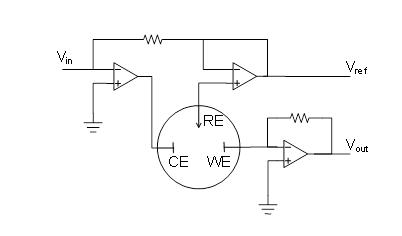
Figure 4.5. Potentiostatic three-electrode set-up. The current flowing through the cell is obtained from Vout.
In principle, the counter electrode in three-electrode set-up can be made of any conductive material as long as its electrochemical behavior does not affect the function of the working electrode. Typical materials for counter electrodes are platinum or graphite. The counter electrode should be placed in the cell in such a way that the products from the reaction on it are not be able to reach the working electrode and affect the reactions taking place there. In practice, this is not a problem due to the slow diffusion of these products, and it is not necessary to place the counter electrode in a separate compartment. The area of the counter electrode needs to be large compared to the area of the working electrode to prevent the reactions at the counter electrode from being the current-determining reactions in the cell.
The reference electrode has to be placed close to the working electrode in order to minimize ohmic losses. This can be achieved by using a Luggin capillary (Figure 4.6.). In this set-up, the reference electrode, for example the Ag/AgCl electrode previously introduced, is placed in a glass capillary that has a narrow tip (Luggin capillary). The capillary is usually filled with the solution being studied. The reference electrode is placed next to the working electrode via this narrow tip. As the distance between the tip and the working electrode is very small, the ohmic drop between the reference electrode and the working electrode is small. The ideal location of a Luggin capillary at the working electrode needs to be experimentally investigated, and it should be kept constant in the measurements. The Luggin capillary should be very close to the working electrode but not touch it.
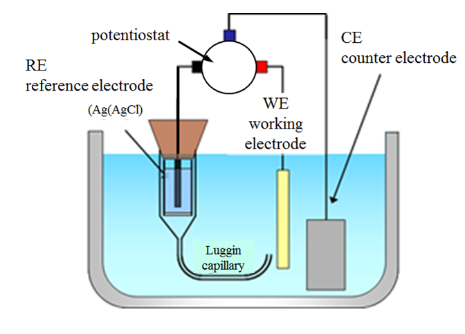
Figure 4.6 Three-electrode set-up.
The device used to carry out electrochemical measurements is called a potentiostat. A potentiostat is based on the circuit presented in Figure 4.5. A potentiostat can be switched to the galvanostatic mode, where the current flowing through the working electrode is controlled and the potential of the working electrode with reference to the reference electrode is measured. Potentiostats offer means to tackle ohmic losses, usually either the ohmic losses in the cell can be measured or it is possible to compensate for them electronically by means of a positive feedback loop.
5. Electrical double layer and adsorption
In electrochemical reactions, there is always an electron transfer step, which takes place at the interface of two phases, for example at the interface of an electrode and electrolyte solution. This interface is studied in greater detail in this chapter.
At the interface of the two phases, there is an interfacial zone, the properties of which are significantly different from those of the inner part of the phase. From an electrochemical point of view, it is important to note that the electrical properties of the interface also differ from those of the bulk phase. If the interfacial region carries a charge, the charge concentrates at the interface. The orientation of the dipole molecules at the interface can also have an effect on the electrical properties of the interface. Furthermore, the adsorption of the dipole molecules or ions on the interface can enhance the accumulation of charges. This charge excess is due to the electrons, ions and dipoles, and generates an electric field. The region in which the charges are located is called the double layer.
When oppositely charged ions and dipoles accumulate on the surface of a charged electrode in an electrolyte solution, a double layer as depicted in Figure 5.1 is formed. The surface properties of the electrode differ from those of the inner phase of the electrode because of the charge excess or deficit with respect to the bulk of the electrode. This interfacial zone on both sides of the phase boundary is called the electrical double layer.
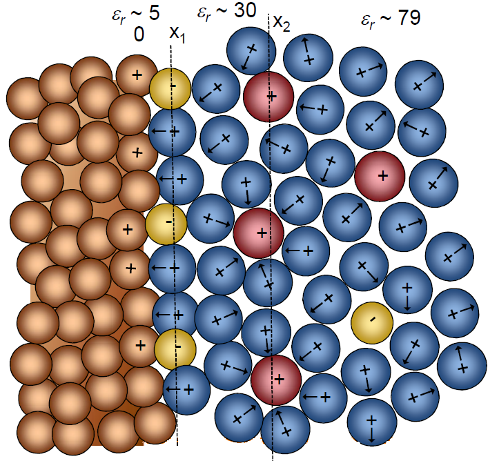
Figure 5.1. Structure of an electrical double layer in an electrolyte solution, when the solution is in contact with a charged electrode. The ions with the solvation layer are closest to the interface at the outer Helmholtz layer (x2), whereas the specifically adsorbed ions at the inner Helmholtz layer (x1) are desolvated.
The solution in the region of the double layer is thought to be made up of several layers. The structure of these layers is affected by the finite size of the ions and molecules, electrostatic forces, mixing entropy, and thermal motion, which reduces the level of organization of the species. The layer closest to the interface is called the inner Helmholtz plane (Figure 5.1). The inner Helmholtz plane consists of specifically adsorbed molecules and ions. Species that are specifically adsorbed are affected by not only electrostatic interactions but also chemical interactions between the surface and the species. The specifically adsorbed species are typically anions, solvent molecules or other neutral molecules. Cations, on the other hand, are very seldom specifically adsorbed. The inner Helmhotz plane is located at the electrical centers of the specifically adsorbed ions.
The outer Helmholtz plane (OHP) is thought to be located at the electrical centers of the closest solvated ions near to the electrode surface. These ions are said to be nonspecifically adsorbed, and the interaction of the solvated ions with charged metal surface involves only long-range electrostatic forces. Their interaction is therefore in principle independent of the chemical properties of the ions.
The region extending from the outer Helmholtz plane to the bulk of the solution is called the diffuse double layer, where the species are organized by thermal motion and the electrostatic force, which gets weaker as the distance from the interface increases. The boundary between the diffuse layer and the bulk of the solution is therefore not well defined. The thickness of the diffuse layer depends on the total ionic strength and is of the order of magnitude10-100 \( \mu \)m.
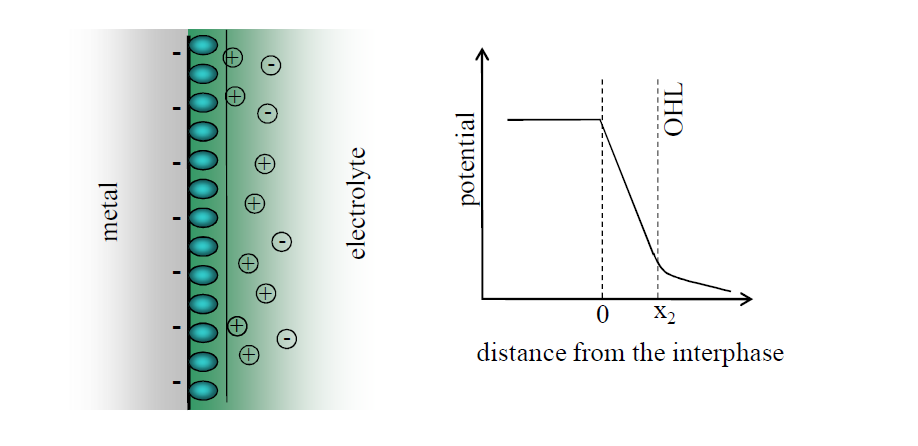 |
a |
|---|---|
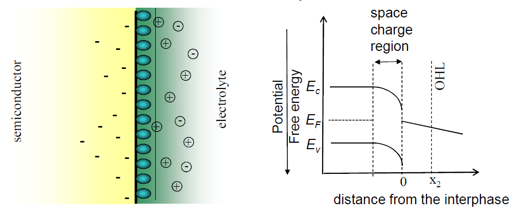 |
b |
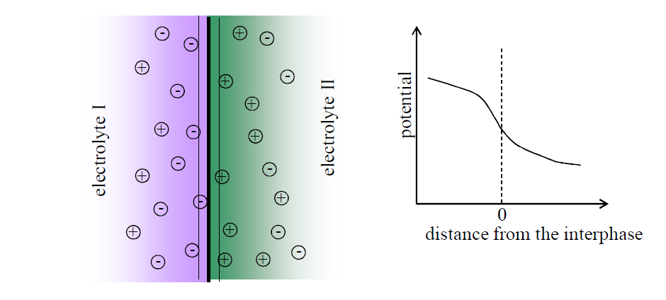 |
c |
Figure 5.2. Structure of electrical double layer and potential distribution at a) the metal electrode-electrolyte interface, b) the semiconductor-electrolyte interface, and c) the interface of two immiscible electrolyte solutions without specifically adsorbed species. Note that in the latter case there is no layer of organized solvent ions at the interface, according to Verwey and Niessen model.
The structure of the electrical double layer and the potential distribution at a) the metal electrode-electrolyte interface, b) the semiconductor-electrolyte interface, and c) the interface of two immiscible electrolyte solutions without specifically adsorbed species is shown in Figure 5.2. At the surface of a semiconductor, the charges are distributed more widely compared to the surface of a metal electrode. At the interface of two immiscible liquids, there is no layer of organized solvent molecules.
5.1. Gibbs adsorption isotherm
Adsorption on electrode surfaces can take place with or without simultaneous charge transfer between the adsorbing species and the electrode. When charge transfer is involved, it can be either partial or complete charge transfer. In this chapter, we look at adsorption, which takes place without charge transfer. The best tool for this is thermodynamics.
Consider an interface of surface area A separating two phases, \( \alpha \) and \( \beta \). These two phases can be, for example, a metal electrode and an electrolyte solution, or two immiscible liquids in contact with one another. In a system with several components, the (electro) chemical potential of each component has to be equal in both phases and at the interface. Experience has shown that real systems tend to either minimize or maximize the interfacial area. Because of this, the free energy of the system has to depend on the area:
| \( \displaystyle dG=\left(\frac{\partial G}{\partial T}\right)dT+\left(\frac{\partial G}{\partial P}\right)dP+\left(\frac{\partial G}{\partial A}\right)dA+\sum\limits_{i}\left(\frac{\partial G}{\partial n_i}\right)_idn_i \) | (5.1) |
|---|
We can give a name to the partial derivative \( (\partial G/\partial A) \): it is the surface tension \( \gamma \). The forces that bind particles together are weaker at the interface because the particles at the surface have fewer neighboring atoms compared to the ones in the bulk. Instead, the particles at the surface interact with particles in the neighboring phase. This changes the equilibrium of forces and can lead to a new force called surface tension. Surface tension is therefore a force at the interface that tends to increase or decrease the growth of the surface. It is significant only in a very thin zone, a few molecules thick, near the interface.
Gibbs energy differentials \( \alpha \) and \( \beta \) are
| \( \displaystyle dG^{\alpha}=\left(\frac{\partial G^{\alpha}}{\partial T}\right)dT+\left(\frac{\partial G^{\alpha}}{\partial P}\right)dP+\sum\limits_{i}\left(\frac{\partial G^{\alpha}}{\partial n_i^{\alpha}}\right)_idn_i^{\alpha} \) | (5.2) |
|---|---|
| \( \displaystyle dG^{\beta}=\left(\frac{\partial G^{\beta}}{\partial T}\right)dT+\left(\frac{\partial G^{\beta}}{\partial P}\right)dP+\sum\limits_{i}\left(\frac{\partial G^{\beta}}{\partial n_i^{\beta}}\right)_idn_i^{\beta} \) | (5.3) |
We will only look at experiments conducted at constant temperature and
pressure, and thus the two first terms of the Gibbs equation can be neglected. Since the phases are in equilibrium, the chemical potentials of each species are
equal in the whole system:
| \( \displaystyle\left(\frac{\partial G}{\partial n_i}\right)=\left(\frac{\partial G^{\alpha}}{\partial n_i^{\alpha}}\right)=\left(\frac{\partial G^{\beta}}{\partial n_i^{\beta}}\right)=\mu_i \) | (5.4) |
|---|
Subtracting the Gibbs energies of phases \( \alpha \) and \( \beta \), the Gibbs energy of the surface is:
| \( \displaystyle dG^{\sigma}=\gamma dA+\sum\limits_i\mu_id(n_i-n_i^{\alpha}-n_i^{\beta}) \) | (5.5) |
|---|
There is either an excess or a deficit of components on the surface compared to the bulk of the solution. The difference in the amounts of substance on the surface and in the bulk is called the surface concentration, or surface excess, \( n_i^{\sigma} \):
| \( \displaystyle n_i^{\sigma}=n_i-n_i^{\alpha}-n_i^{\beta} \) | (5.6) |
|---|
Consider a situation in which a surface is formed slowly between two phases from zero to a finite value A, while pressure, temperature, and the composition of the solution are constant. In this case, the surface concentration increases from zero to the value \( n_i^{\sigma} \), but \( \gamma \) and \( \mu_i \) are constant. Equation (5.6) is substituted into Equation (5.5) and integrated
| \( \displaystyle dG^{\sigma}=\gamma dA+\sum\limits_i\mu_idn_i^{\sigma} \) |
(5.7) |
|---|---|
| \( \displaystyle\int_{0}^{G^{\sigma}}{dG^{\sigma}}=\gamma \int_{0}^{A}{dA} +\sum\limits_i\mu_i \int_{0}^{n_i^{\sigma}}{dn_i^{\sigma}} \) | (5.8) |
And we obtain
| \( \displaystyle G^{\sigma}=\gamma dA+\sum\limits_i\mu_in_i^{\sigma} \) | (5.9) |
|---|
The total differential of Gibbs energy is
| \( \displaystyle dG^{\sigma}=\gamma dA+\sum\limits_i\mu_in_i^{\sigma}+Ad\gamma+\sum\limits_in_i^{\sigma}d\mu_i \) | (5.10) |
|---|
Equations (5.7) and (5.10) have to be equivalent, and thus the sum of the last two terms of Equation (5.10) is zero.
| \( \displaystyle Ad\gamma+\sum\limits_in_i^{\sigma}d\mu_i=0 \) | (5.11) |
|---|
It is often convenient to talk about surface excess per unit area. We therefore define the surface concentration \( \Gamma_i=n_i^{\sigma}/A \) , and the previous equation becomes
\( \displaystyle -d\mu_1\=\sum\limits_i\Gamma_id\mu_i \) |
(5.12) |
|---|
This equation is called the Gibbs adsorption isotherm. The equation implies that measurements of surface tension will give us information on the structure of the interface.
It is useful to describe the adsorption of other components with respect to one predominant component, e.g. a solvent, in dilute solutions in particular. Here, the main component is given the subscript 1. In the bulk of the solution, the Gibbs-Duhem equation holds. According to it, for any phase at constant temperature and pressure, the following is true:*
| \( \displaystyle\sum\limits_in_id\mu_i=0 \) | (5.13) |
|---|
The change in the electrochemical potential of the main component is therefore
| \( \displaystyle -d\mu_1=\sum\limits_{i \neq1} \frac{n_i}{n_1}d\mu_i \) | (5.14) |
|---|
Using this, the Gibbs adsorption isotherm gives
| \( \displaystyle -d\gamma=\sum\limits_{i\neq 1} \Gamma_id\mu_i+\Gamma_1d\mu_1=\sum\limits_{i\neq 1}\left(\Gamma_i-\frac{n_i}{n_1}\Gamma_1\right)d\mu_i \) | (5.15) |
|---|
The bracketed term is called the relative surface excess \( \Gamma^{\sigma} \)
| \( \displaystyle\Gamma_i^{\sigma}=\Gamma_i-\frac{n_i}{n_1}\Gamma_1 \) | (5.16) |
|---|
In very dilute solutions n1 » ni, and \( \Gamma_i^{\sigma} \approx \Gamma_i \).
5.2. Electrocapillary equation
Electric charges affect the surface tension of the interface of two phases. If one of these phases is a metal and another is an electrolyte solution, the phenomenon is called electrocapillarity.
The surface tension of an ideally polarizable electrode (see Chapter 1.3.4) always depends on the potential. To understand the dependency of surface tension, composition, and cell potential, consider a situation where one of the electrodes is ideally nonpolarizable. The potential of this reference electrode is therefore constant, and the change in the cell potential has an effect on the interface of the working electrode and the electrolyte. The working electrode must be ideally nonpolarisable.
Let us look at a cell, in which a hydrogen electrode is the ideally nonpolarizable reference electrode and a mercury electrode is the ideally polarizable working electrode. The electrolyte in the cell is an aqueous solution of hydrogen chloride.
| Pt(s) | H2(g) | HCl(aq) | Hg(l) | Pt(s) | (5.17) |
|---|
As we showed in Chapter 2, the chemical potentials can be replaced by the electrochemical potentials of ions. In the bulk of the solution, the electroneutrality condition cancels the potential terms out, but there is an excess of charge at the interface, in other words a local deviation from the electroneutrality condition. Applying the Gibbs adsorption isotherm (5.12) to the interface of HCl-Hg using the relative surface excesses with respect to water (5.16), we obtain
| \( \displaystyle -d\gamma=\left(\Gamma_{\text{Hg}^+}^{\sigma}d\tilde\mu_{\text{Hg}^+}+\Gamma_{\text{e}^-}^{\sigma}d\tilde\mu_{\text{e}^-}^{\text{Hg}}\right)+\left(\Gamma_{\text{H}^+}^{\sigma}d\tilde\mu_{\text{H}^+}+\Gamma_{\text{Cl}^-}^{\sigma}d\tilde\mu_{\text{Cl}^-}\right) \) | (5.18) |
|---|
There is an equilibrium between the metal ions and electrons in mercury and between the ions and molecules in the electrolyte. Thus
| \( \displaystyle\mu_{\text{Hg}}=\tilde\mu_{\text{Hg}}=\tilde\mu_{\text{Hg}^+}+\tilde\mu_{\text{e}^-}^{\text{Hg}} \) |
(5.19) | |
|---|---|---|
|
(5.20) |
The excess of charges at the interface of metallic mercury and the electrolyte, \( \sigma \)m and \( \sigma \)s can be expressed as
| \( \displaystyle\sigma^m=\sum\limits_iz_iF\Gamma_i^{\sigma}=F\left(\Gamma_{\text{Hg}^+}^{\sigma}-\Gamma_{\text{e}^-}^{\sigma}\right) \) |
(5.21) |
|---|---|
| \( \displaystyle\sigma^s=-\sigma^m=F\left(\Gamma_{\text{H}^+}^{\sigma}-\Gamma_{\text{Cl}^-}^{\sigma}\right) \) | (5.22) |
Substituting Equations (5.19)-(5-22) into Equation (5.18) we obtain
| \( \displaystyle -d\gamma=\Gamma_{\text{Hg}^+}^{\sigma}d\mu_{\text{Hg}}+\Gamma_{\text{Cl}^-}^{\sigma}d\mu_{\text{HCl}}-\frac{\sigma^m}{F}\left(d\tilde\mu_{\text{H}^+}^{\text{HCl}}+d\tilde\mu_{\text{e}^-}^{\text{Hg}}\right) \) | (5.23) |
|---|
Based on the equilibrium conditions at the phase boundaries, we can write
| \(\displaystyle \tilde\mu_{\text{e}^-}^{\text{Hg}}=\tilde\mu_{\text{e}^-}^{\text{Pt,w}} \) |
(5.24) |
|---|---|
| \( \displaystyle\tilde\mu_{\text{e}^-}^{\text{H}_2}=\tilde\mu_{\text{e}^-}^{\text{Pt,r}} \) |
(5.25) |
| \( \displaystyle\tilde\mu_{\text{H}^+}^{\text{H}_2}=\tilde\mu_{\text{H}^+}^{\text{HCl}} \) |
(5.26) |
where superscript w denotes the working electrode and r the reference electrode. On the other hand, the composition of gas in the hydrogen phase of the reference electrode is constant and because of the equilibrium H2 \(\ce{ <=> }\) 2 H+ + 2 e– we have
| \( \displaystyle\tilde\mu_{\text{H}^+}^{\text{H}_2}=-\tilde\mu_{\text{e}^-}^{\text{H}_2} \) | (5.27) |
|---|
Applying the definition of potential E
| \( dG=-nFdE \) | (5.28) |
|---|
The last term of Equation (5.23) can be written as
| \( -\displaystyle\frac{\sigma^m}{F}(d\tilde\mu_{\text{e}^-}^{\text{Pt,w}}+\tilde\mu_{\text{e}^-}^{\text{Pt,r}})=\sigma^mdE \) | (5.29) |
|---|
Thus,
| \( \displaystyle -d\gamma=\Gamma_{\text{Hg}^+}^{\sigma}d\mu_{\text{Hg}}+\Gamma_{\text{Cl}^-}^{\sigma}d\mu_{\text{HCl}}+\sigma^mdE \) | (5.30) |
|---|
This is called the electrocapillary equation. The name is of historic origin, derived from the early application of the equation to the determination of surface tension at mercury-electrolyte interfaces. The equation implies that varying the concentration and following the change in the surface tension at constant potential, the surface concentrations of ions can be determined. On the other hand, if the change in potential is followed when the composition of the solution is constant, the surface charge \( \sigma \)m can be found.
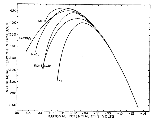
Figure 5.3. Electrocapillary curves, i.e. surface tension of mercury electrode as a function of potential in various electrolytes. The potential is plotted with respect to the potential of zero charge for NaF. D.C. Grahame, Chem. Rev. 41 (1947) 441.
Figure 5.3 shows the nearly parabolic shape typical of electrocapillary curves which describe the surface tension as a function of potential for electrolyte solutions in contact with the mercury electrode. If the mercury is pure, \( \mu \)Hg = 0 and d\( \mu \)Hg = 0. Also, d\( \mu \)HCl = 0, if the concentration of the acid is assumed to be constant. In this case, the previous equation becomes
| \( \displaystyle\left(\frac{d\gamma}{dE}\right)_{P,T,\mu_{\text{HCl}}}=-\sigma^m \) | (5.31) |
|---|
It is evident that the slope of the tangent to the electrocapillary curve gives the magnitude of the excess charge at any potential.
Even though the curves for each solution are substantially different from each other, we can observe a common feature in all curves: the existence of a maximum surface tension. The corresponding potential is the potential of zero charge (PZC), where \( \sigma \)m = \( \sigma \)s = 0. At more negative potentials, the surface of the electrode has a negative excess charge, and at more positive potentials the surface charge is positive. The charge at the surface weakens surface tension because like charges tend to repel each other.
Neutral organic molecules are typically best adsorbed close to the potential of zero charge because at PZC the polar water molecules in the inner Helmhotz plane are less organized and neutral molecules can more easily penetrate the inner parts of the double layer. The surface coverage varies as a function of potential. The surface coverage \( \theta \) is the fraction of the electrode surface that is covered by molecules (0 < \( \theta \) < 1). If the molecules are specifically adsorbed, the previous model is not valid and the surface coverage can be independent of the potential.
The capacitance of the double layer per unit area C is the derivative of the excess charge with respect to the potential at constant composition
| \( \displaystyle C_{dl}=\left(\frac{\partial\sigma^m}{\partial E}\right)_{\mu,T} \) | (5.32) |
|---|
5.3. Gouy-Chapman model
The classic Gouy-Chapman model describes the layer between the outer Helmholtz plane and the bulk of the solution. In this layer, the charges are assumed to be point charges and the solution is a medium without a structure described by the relative permittivity \( \varepsilon \)r. Since the only thing that matters is the potential difference, the potential of the bulk solution can be assumed to be zero and the potential of the Helmholtz plane is denoted \( \phi \)2. Let us leave the inner layer for a moment and take a closer look at the diffuse layer.
The total charge density r(x) is obtained from electrostatics using the Poisson equation:
| \( \displaystyle\rho(x)=-\varepsilon_r\varepsilon_0\frac{d^2\phi}{dx^2} \) | (5.33) |
|---|
On the other hand, the charge density can be expressed as the sum of all ions present in the diffuse layer:
| \( \displaystyle\rho(x)=\sum_iz_iFc_i(x)\) | (5.34) |
|---|
The ions in the double layer follow the Boltzmann distribution:
| \( \displaystyle c_i(x)=c_i^b\exp\left(-\frac{z_iF\phi}{RT}\right) \) | (5.35) |
|---|
Combing the two equations, we get the Poisson-Boltzmann differential equation:
| \( \displaystyle\frac{d^2\phi}{dx^2}=-\frac{F}{\varepsilon_r\varepsilon_0}\sum\limits_iz_ic_i^b\exp\left(-\frac{z_iF\phi}{RT}\right) \) |
(5.36) |
|---|
Intergration by substitution gives
| \(\displaystyle \frac{d\phi}{dx}=p \Rightarrow \frac{d^2\phi}{dx^2}=\frac{dp}{dx}=\frac{dp}{d\phi}\frac{d\phi}{dx}=p\frac{dp}{d\phi} \) | (5.37) |
|---|
Thus
| \( \displaystyle\int pdp=-\frac{F}{\varepsilon_r\varepsilon_0}\int\sum\limits_iz_ic_i^b\exp\left(-\frac{z_iF\phi}{RT}\right)d\phi \) |
(5.38) |
| \( \displaystyle\frac{1}{2}\left(\frac{d\phi}{dx}\right)^2=\frac{RT}{\varepsilon_r\varepsilon_0}\sum\limits_iz_ic_i^b\exp\left(-\frac{z_iF\phi}{RT}\right)+B \) | (5.39) |
|---|
The integration constant B can be determined with the help of the following boundary conditions: The electric field must vanish in the bulk solution, and thus this symmetry requirement results in a boundary condition d\( \phi \)/dx = 0. According to the electroneutrality condition, the net charge of the bulk must also be zero, and therefore \( \phi \) = 0. Equation (5.39) therefore becomes
| \( \displaystyle\frac{1}{2}\left(\frac{d\phi}{dx}\right)^2=\frac{RT}{\varepsilon_r\varepsilon_0}\sum\limits_iz_ic_i^b\left[\exp\left(-\frac{z_iF\phi}{RT}\right)-1\right] \) | (5.40) |
|---|
Consider a symmetrical electrolyte, e.g. NaCl (1:1) or CaCO3 (2:2). Equation (5.40) becomes now
| \( \displaystyle\left(\frac{d\phi}{dx}\right)^2=\frac{2RTc^b}{\varepsilon_r\varepsilon_0}\left[\exp\left(\frac{-zF\phi}{RT}\right)+\exp\left(\frac{zF\phi}{RT}\right)-2\right]=\frac{8RTc^b}{\varepsilon_r\varepsilon_0}\sinh^2\left(\frac{zF\phi}{2RT}\right) \) |
(5.41) |
| \( \displaystyle\Rightarrow \frac{d\phi}{dx} =-\left(\frac{8RTc^b}{\varepsilon_r\varepsilon_0}\right)^{1/2}\sinh\left(\frac{zF\phi}{2RT}\right) \) | (5.42) |
|---|
Note that we need to choose the negative root for (d\( \phi \)dx)! The equation can be integrated in a closed form, and after some slightly tedious algebra, the solution becomes
| \( \displaystyle\frac{\tanh(zF\phi/4RT)}{\tanh(zF\phi_0/4RT)}=\exp(-\kappa x) \) | (5.43) |
|---|
where \( \phi \)0 is potential at the electrode surface (x = 0) and
| \( \displaystyle\kappa=\left(\frac{2c^bz^2F^2}{\varepsilon_r\varepsilon_0RT}\right)^{1/2} \) | (5.44) |
|---|
is again the Debye length (see also Equation (2.33)). The potential profile (5.43) is not very illustrative and because of that, the tanh terms are usually linearized, tanh(x) ≈ x. The linearized result is simply
| \( \displaystyle\phi(x)=\phi_0e^{-\kappa x} \) | (5.45) |
|---|
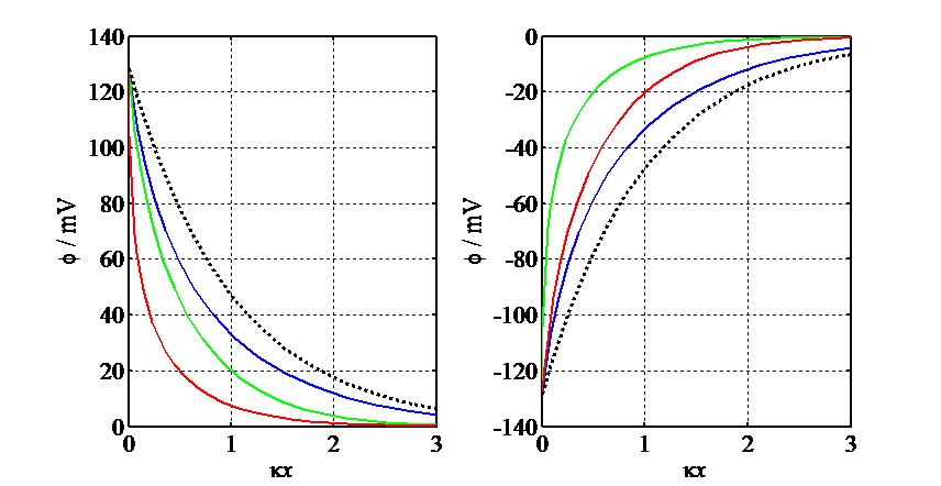
Figure 5.4. Simulated potential profiles according to Gouy-Chapman theory, F\( \phi \)0/RT = ±5: 1:1 electrolyte (blue), 2:1 electrolyte (green), 1:2 electrolyte (red). The black broken line describes the linearized equation (5.44). When \( \phi \)0 > 0, the curve for the 2:2 electrolyte almost merges with the curve for the 1:2 electrolyte (red) and when \( \phi \)0 < 0, the curve for the 2:1 electrolyte (green). Note the order of the curves with respect to \( \phi \)0.
The potential profiles are shown in Figure 5.4, including for the unsymmetrical electrolytes obtained by integrating Equation (5.40) numerically. In Figure 5.4, \( \kappa \) = (2cbF2/\( \varepsilon \)r\( \varepsilon \)0RT)1/2.
In aqueous solution at 25 ºC, the Debye length is \( \kappa \)–1 ≈ 10–9 (z2cb)–1/2(mol/cm)1/2. A good rule of thumb is that in 1.0 mM solution, for 1:1 electrolyte \( \kappa \)–1 ≈ 10 nm.
According to Gauss's law, the charge q inside the volume V is
| \( \displaystyle q=\varepsilon_r\varepsilon_0 \oint{E} \cdot dS \) | (5.46) |
|---|
where E is the electric field through a surface S. In our one-dimensional case, the scalar product E·dS is zero at all points except on the electrode surface, where it is (d\( \phi \)/dx)0dS. The charge density of the double layer is therefore
| \( \displaystyle q=\varepsilon_r\varepsilon_0\left(\frac{d\phi}{dx}\right)_0 \) |
(5.47) |
|---|
The charge density of the electrode for a symmetrical electrolyte is
| \( \displaystyle\sigma^m=-q=(8RTc^b\varepsilon_r\varepsilon_0)^{1/2}\sinh\left(\frac{zF\phi_0}{2RT}\right) \) |
(5.48) |
|---|
The differential capacitance of the electrode therefore becomes
| \( \displaystyle C_d=\frac{\partial\sigma^m}{\partial\phi_0}=\left(\frac{2c^bz^2F^2\varepsilon_r\varepsilon_0}{RT}\right)^{1/2}\cosh\left(\frac{zF\phi_0}{2RT}\right) \) |
(5.49) |
|---|
The scaled differential capacitances are shown in Figure 5.5, including for the unsymmetrical electrolytes. Even though the potential profiles cannot be determined in a closed form, the capacitances can be calculated using Equations (5.40) and (5.47).
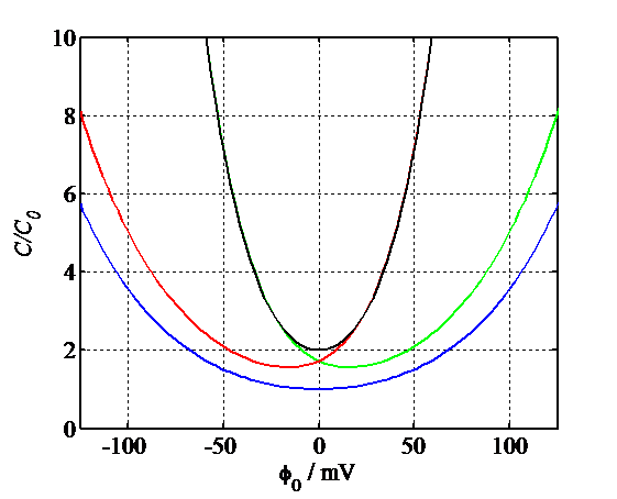
Figure 5.5. Simulated capacitances according to Gouy-Chapman theory: 1:1 electrolyte (blue), 2:1 electrolyte (green), 1:2 electrolyte (red), 2:2 electrolyte (black).
The scaled capacitances for 1:1 electrolytes are:
| \( \displaystyle C_d/C_0=\cosh(\varphi_0/2) \) |
(5.50a) |
|---|
For a 2:1 electrolyte:
| \( \displaystyle\frac{C_d}{C_0}=\frac{e^{\varphi_0}-e^{-2\varphi_0}}{\sqrt{2e^{\varphi_0}-3+e^{-2\varphi_0}}} \) | (5.50b) |
|---|
For a 1:2 electrolyte:
| \( \displaystyle\frac{C_d}{C_0}=\frac{e^{2\varphi_0}-e^{-\varphi_0}}{\sqrt{e^{2\varphi_0}-3+2e^{-\varphi_0}}} \) | (5.50c) |
|---|
And for a 2:2 electrolyte:
| \( \displaystyle C_d/C_0=2\cosh(\varphi_0) \) |
(5.50d) |
| \( \displaystyle C_0=\left(\frac{2F^2c^b\varepsilon_0\varepsilon_r}{RT}\right)^{1/2} \) ; \( \varphi=\frac{\phi}{RT} \) |
(5.51) |
|---|
5.4. Effect of inner layer on capacitance
As shown in Figure 5.1, the surface of an electrode includes an inner and an outer Helmholtz layer, which may have a net charge. In the mathematical treatment of the diffuse double layer, \( \phi \)0 must be replaced by \( \phi \)2 and x by \( x-x_2 \) in the previous equations; keep in mind that x2 is the distance between the outer Helmholtz plane and the electrode, and \( \phi \)2 = \( \phi \)(x2). From now on, we will treat the Helmholtz layers as one and call this the inner layer.
Continuity of electric flux is one of the central laws of electrostatics. According to it, at the phase boundary \( \alpha \)| \( \beta \), we have
| \( \displaystyle\varepsilon_r^{\alpha}\varepsilon_0\left(\frac{\partial\phi^{\alpha}}{\partial x}\right)-\varepsilon_r^{\beta}\varepsilon_0\left(\frac{\partial\phi^{\beta}}{\partial x}\right)=q \) | (5.52) |
|---|
Superscripts \( \alpha \) and \( \beta \) in Equation (5.52) denote the respective phases, and q is the charge density of the phase boundary. If q is zero, and \( \varepsilon_r^{\alpha}=\varepsilon_r^{\beta} \), the continuity condition of electric flux means that the electric field is continuous.
Assume that the charge of the inner layer is zero. It follows that the potential profile, according to the Poisson equation, is linear:
| \(\displaystyle \left(\frac{\partial\phi}{\partial x}\right)_{\text{inner layer}}=\frac{\phi_2-\phi_0}{x_2} \) | (5.53) |
|---|
Because of the partial loss of degrees of freedom of the water molecules in the inner layer, its relative permittivity is low compared to that of the bulk solution. Based on Equations (5.42), (5.48) and (5.52), the continuity condition of the electric flux density between the layers at the boundary at x = x2 for a symmetrical z:z electrolyte becomes
| \( \displaystyle\sigma^m=-\varepsilon_r\varepsilon_0\frac{\phi_2-\phi_0}{x_2} =(8RTc^b\varepsilon_r^b\varepsilon_0)^{1/2}\sinh\left(\frac{zF\phi_0}{2RT}\right) \) | (5.54) |
|---|
where \( \varepsilon \)r is the relative permittivity of the inner layer, and \( \varepsilon \)rb that of the bulk solution. We can now solve this for \( \phi \)2:
| \(\displaystyle \phi_2=\phi_0-\frac{\sigma^mx_2}{\varepsilon_r\varepsilon_0} \) | (5.55) |
|---|
Substituting \( \phi \)2 into Equation (5.54) and taking the derivative with respect to \( \phi \)0 results, after some algebra, in the total capacitance of the electrode, CT:
| \( \displaystyle\frac{1}{C_{\text{T}}}=\left(\frac{\partial\sigma^m}{\partial\phi_0}\right)^{-1}=\frac{x_2}{\varepsilon_r\varepsilon_0}+\frac{1}{(2\varepsilon_r^b\varepsilon_0z^2F^2c_b/RT)\cosh(zF\phi_2/2RT)}=\frac{1}{C_2}+\frac{1}{C_d} \) | (5.56) |
|---|
Equation (5.56) states that the total capacitance is made up of two components, the series combination of the inner layer and the diffuse layer. [1] The capacitance of the inner layer C2 is independent of potential:
| \(\displaystyle C_2=\frac{\varepsilon_r\varepsilon_0}{x_2} \) | (5.57) |
|---|
Because C2 » Cd, Cd dominates the total capacitance. The analysis can even be taken a step further: The charge of the electrode \( \sigma \)m in Equation (5.32) can be solved by integration:
| \(\displaystyle \sigma^m=\int_{E_{pzc}}^E {C_ddE} \) | (5.58) |
|---|
where Epzc is the potential of zero charge of the electrode, in other words, the potential at which \( \sigma \)m = 0. The potential of zero charge is usually taken to be the potential at which the capacitance of the electrode is at the minimum. Without specific adsorption, i.e. the charge of the inner layer, Epzc ≈ 0. The non-zero minimum of capacitance is therefore considered to be the first signal of specific adsorption. The integral (5.58) must be solved numerically from the experimental capacitance curve because its mathematical form is not known.
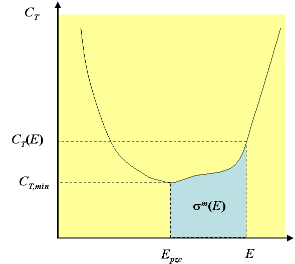
Typically, however, there are specifically adsorbed ions on the electrode. In this case, the charge of the electrode \( \sigma \)m is compensated for the charge of the inner layer
----
[1] In parallel combination, the values of capacitance are added, and in series, the reciprocals of the values, see Chapter 9.
[2] If \( \varepsilon \)r ≈ 5 and x2 ≈ 1 nm, C2 ≈ 44 mFcm-2, whereas Cd is typically of the order of magnitude 0.1...1 mFcm-2.
You can now test your conceptual knowledge by taking Quiz Chapter 5.
6. Electrochemical reaction kinetics
Like all heterogeneous processes, an electrochemical reaction consists of several reaction steps. First, a reactant must be transported to the electrode surface; that was considered in Chapter 3. Prior to a reaction, a reactant may be adsorbed on the surface and the adsorbed species undergoes electron transfer. A reaction product must desorb from the surface and be transported away, in order to yield to other species to react. The effect of adsorption on the reaction rate has been considered in Chapter 5 and 9, while this Chapter concentrates on the rate and mechanisms of electron transfer.
An electrochemical reaction has the special feature that its rate can be externally controlled in situ by varying the electrode potential or electric current. This is possible because of Faraday’s law (see Chapter 1), which states that the reaction rate is proportional to the electric current. The core of an electrochemical reaction is electron transfer that is basically a quantum mechanical phenomenon but is traditionally modeled analogously to the activated complex theory14F*
*Rudolph Marcus received the Nobel prize in chemistry in 1992 for his theory of electron transfer, known as the Marcus theory; it will be addressed briefly later.
6.1. Reaction rate via the free energy model
Let us consider a redox reaction
| \( \displaystyle\text{O}+n\text{e}^- \)\(\ce{ <=> }\)\( \text{R} \) | (6.1) |
|---|
where n electrons are transferred to the oxidized species ’O’, forming the reduced species ’R’. At equilibrium, the following equation applies:
| \(\displaystyle \mu_{\text{R}}^0+RT\text{ln}a_{\text{R}}+z_{\text{R}}F \phi^w= \mu_{\text{O}}^0+RT\text{ln}a_{\text{O}}+z_{\text{O}}F \phi^w+n(\mu_{\text{e}}^0+RT\text{ln}a_{\text{e}}-F \phi^{\text{M}}) \) | (6.2) |
|---|
where \( \phi^w \) is the Galvani potential in the aqueous phase and \( \phi^{\text{M}} \) that of an electron (in the electrode); the other variables are defined in Chapter 2. The activity of an electron in the solid electrode (most commonly a metal) ae = 1, and n = zO - zR. Hence, rearranging Equation (6.2), the Nernst equation is obtained:
| \( \displaystyle\phi^{\text{M}}-\phi^{\text{w}}=\Delta\phi_{eq}=-\frac{\Delta G^0}{nF}+\frac{RT}{nF}\text{ln} \left(\frac{a_{\text{O}}}{a_{\text{R}}}\right)_{eq}=\Delta\phi^0+\frac{RT}{nF}\text{ln}\left(\frac{a_{\text{O}}}{a_{\text{R}}}\right)_{eq} \) | (6.3) |
|---|
where
| \( \displaystyle\Delta G^0=\mu_{\text{R}}^0-\mu_{\text{O}}^0-n\mu_{\text{e}}^0 \) | (6.4) |
|---|
When the electrode potential \( \phi^{\text{M}} \) is changed, it follows that
| \( \displaystyle nF(\Delta\phi-\Delta\phi_{eq})=(RT\text{ln}a_{\text{O}}-RT\text{ln}a_{\text{O}, eq})-(RT\text{ln}a_{\text{R}}-RT\text{ln}a_{\text{R}, eq})=\Delta\mu_{\text{O}}-\Delta\mu_{\text{R}} \) | (6.5) |
|---|
In other words, the change in the electrode potential is converted to a change in the chemical potentials of the species residing in the solution phase.
The Nernst equation contains the activities of the species involved in the reaction, but the estimation of their activity coefficients is not always easy. Fortunately, the ratio of the activity coefficients approaches unity much faster than the individual coefficients. The Nernst equation is therefore most often written in terms of concentrations:
| \( \displaystyle E=E^0+\frac{RT}{nF}\text{ln}\left(\frac{\gamma _{\text{O}}}{\gamma _{\text{R}}}\right)_{eq}+\frac{RT}{nF}\text{ln}\left(\frac{c_{\text{O}}}{c_{\text{R}}}\right)_{eq}=E^{0'}+\frac{RT}{nF}\text{ln}\left(\frac{c_{\text{O}}}{c_{\text{R}}}\right)_{eq} \) | (6.6) |
|---|
In Equation (6.6) the Galvani potential \( \phi \) is replaced by E to emphasize that the electrode potential is measured against some reference value. The quantity E0’ is known as the formal potential. The use of formal potential is also practical because during an electrochemical reaction the concentrations of O and R on the electrode surface change as a function of the electric current, and the formal potential provides one of the boundary conditions of the transport problem. We will look at this in more detain in Chapter 6.2.
The rate of reaction (6.1), r, can be written in the usual form as
| \( \displaystyle r=k_{red}c_{\text{O}}^s-k_{ox}c_{\text{R}}^s \) | (6.7) |
|---|
where kred and kox are the rate constants (cm s-1) of the heterogeneous reduction and oxidation reactions respectively and the superscript ’s’ denotes the surface concentrations. Let’s assume that the rate constants follow the Arrhenius formalism:
| \( \displaystyle k_x=A_xe^{-\Delta G_{x,a}^{\ddagger}/RT} \) \( x=red, ox \) |
(6.8) |
|---|
In Equation (6.8) Ax is the pre-exponential (frequency) factor of reaction x and \( \Delta G_{x,a}^{\ddagger} \)its activation energy. At equilibrium r = 0, viz \( k_{red}c_{\text{O}}^s=k_{ox}c_{\text{R}}^s \), and when E = E0’*, \( c_{\text{O}}^s=c_{\text{R}}^s \). This means that kred = kox and we call this quantity as the standard rate constant k0:
| \( \displaystyle k^0=k_{red}(E=E^{0'})=k_{ox}(E=E^{0'}) \) | (6.9) |
|---|
Figure 6.1 shows a scheme of the free energy profiles at equilibrium (left) and after changing the electrode potential (right); the activation energies or the pre-exponential factors do not need to be equal in both oxidation and reduction reactions, although they are shown this way for the sake of clarity.
When the electrode potential is changed, it can be interpreted as the change of the chemical potential or free energy of either of the species, as previously shown. On the right of Figure 6.1 the electrode potential is raised by \( \Delta E \), raising the free energy of R by \( \Delta G=nF\Delta E \), consequently shifting the reaction equilibrium towards oxidation. The energy barrier of the oxidation reaction does not, however, reduce by \( nF\Delta E \) but, as can be seen in the plot, by the fraction that is denoted \( \alpha nf\Delta E \).† Accordingly, the energy barrier of the reduction reaction is increased by the fraction \( (1- \alpha)nf\Delta E \). The quantity a is known as the charge transfer coefficient. Its value depends on the symmetry of the energy barrier and the electrode potential, taking the value 0.5 in the vicinity of E0’, regardless of the symmetry.
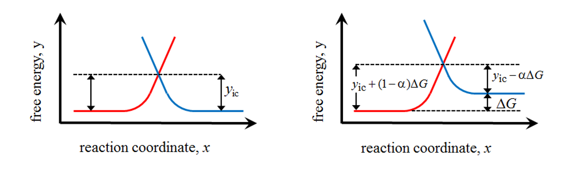
Figure 6.1. Free energy profiles at equilbrium (left) and after changing the electrode potential (right).
The rate constants are according to the Arrhenius formalism\( \displaystyle k_{red}=k^0e^{(\alpha-1)nf(E-E^{0'})} \) and \( k_{ox}=k^0e^{\alpha nf(E-E^{0'})} \) |
(6.10) |
|---|
where f = F/RT. Equations (6.10) are general in the sense that in all approaches the form of the rate constants remains the same, only the the interpretation of the activation energy and the charge transfer coefficient depend on the model applied.‡
Inserting the rate constants from (6.10) into Equation (6.7) at equilibrium (\( r \equiv0 \)), the Nernst equation is restored, i.e. our kinetic model agrees with thermodynamics:
| \( \displaystyle\frac{c_{\text{O}}^s}{c_{\text{R}}^s}=\frac{k_{ox}}{k_{red}}=e^{nf(E-E^{0'})} \) | (6.11) |
|---|
*Since the potential of a single electrode \( \Delta\phi \) cannot be measured, \( E=\Delta\phi+K \) where K is a constant fixing of the potential scale. We therefore use an arbitrary ’E scale’ to emphasize that our treatise is independent of the reference potential, provided that E0’ is defined on the same scale.
† This notation follows the convention used in the following books: K.J. Vetter, Electrochemical kinetics, Academic Press, New York 1967; T, Erdey-Grúz, Kinetics of electrode processes, Adam Hilger, Lontoo 1972.
‡ In the analysis of multistep reaction mechanisms, n denotes the number of electrons transferred in the rate-determining step, often denoted by na, that is nearly always one. In equation (6.12), however, n denotes the total number of electrons transferred in a redox reaction. Obviously, na ≤ n. These issues are relevant in, e.g. oxygen evolution.
6.2. Current-voltage curves
The characteristics of electrochemical reactions is represented best with steady-state current-voltage curves. According to the IUPAC convention, oxidation current is positive. Therefore, using the notation of Equation (6.7) the Faraday law gives (see also Equation (3.3))\( \displaystyle\frac{i}{nF}=k_{ox}c_{\text{R}}^s-k_{red}c_{\text{O}}^s \) |
(6.12) |
|---|
Inserting the dependence of the rate constants on potential it is therefore possible to sketch a current-voltage curve; the only problem comes from the surface concentrations that change as a function of electric current. We begin the analysis with a reversible reaction, i.e. a reaction that has such a high rate that the surface concentrations follow the Nernst equilibrium at all times and in all currents.
6.2.1 Reversible reaction
We consider only the case of a trace ion (see (3.47)) that gives the boundary condition
| \(\displaystyle\frac{i}{nF}=D_{\text{R}}\left(\frac{\partial c_{\text{R}}}{\partial x}\right)_{x=0}=-D_{\text{O}}\left(\frac{\partial c_{\text{O}}}{\partial x}\right)_{x=0} \) | (6.13) |
|---|
In a stationary state (steady state) the diffusion equation (3.53) becomes
| \( \displaystyle\frac{\partial c}{\partial t}=D\frac{\partial^2c}{\partial x^2}=0 \) | (6.14) |
|---|
making concentration profiles linear. As will be explained in Chapter 7, a diffusion boundary layer (DBL) of the thickness \( \delta \) is formed in the vicinity of an electrode. With the boundary condition \( c_i(\delta)=c_i^b(i=\text{R,O}) \) the following result is reached:
| \( \displaystyle\frac{i}{nF}=D_{\text{R}}\frac{c_{\text{R}}^b-c_{\text{R}}^s}{\delta}=D_{\text{O}}\frac{c_{\text{O}}^b-c_{\text{O}}^s}{\delta} \) | (6.15) |
|---|
In Figure 6.2, steady-state concentration profiles during an oxidation reaction are depicted (anodic current, i > 0).
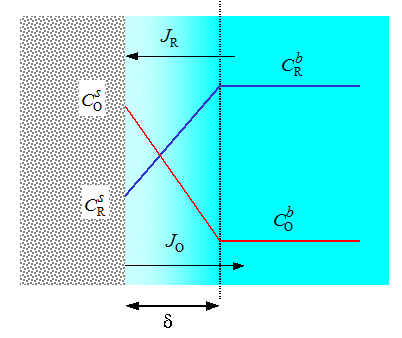
It should be noted that the fluxes of O and R are equal but opposite in direction, JR = -JO, in order to maintain the mass balance, as Equation (6.13) actually also shows. As can easily be seen from the picture, (and Equation (6.15) the highest possible current is obtained when the surface concentration of R reaches zero. This current is called the limiting current. Accordingly, if we consider a reduction reaction, the highest possible cathodic current (i < 0) is obtained when the surface concentration of O reaches zero. The anodic and cathodic current densities are respectively obtained from Equation (6.15):
| \( \displaystyle i_{\text{lim}}^{ox}=nFD_{\text{R}}c_{\text{R}}^b/\delta \) and \( i_{\text{lim}}^{red}=-nFD_{\text{O}}c_{\text{O}}^b/\delta \) |
(6.16) |
|---|
The surface concentrations can be written with the help of current density as:
| \( \displaystyle c_{\text{R}}^s=c_{\text{R}}^b-\frac{i\delta}{nFD_{\text{R}}} \) and \( c_{\text{O}}^s=c_{\text{O}}^b+\frac{i\delta}{nFD_{\text{O}}} \) |
(6.17) |
|---|
From Equation (6.16), the bulk
concentrations can be solved as a function of the limiting current density, as a result of which the following very useful expressions are obtained:
| \( \displaystyle c_{\text{R}}^s=\frac{\left(i_{\text{lim}}^{ox}-i\right)\delta}{nFD_{\text{R}}} \) and \( c_{\text{O}}^s=-\frac{\left(i_{\text{lim}}^{red}-i\right)\delta}{nFD_{\text{O}}} \) |
(6.18) |
|---|
| \( \displaystyle c_{\text{R}}^s=c_{\text{R}}^b\left(1-\frac{i}{i_{\text{lim}}^{ox}}\right) \) and \( c_{\text{O}}^s=c_{\text{O}}^b\left(1-\frac{i}{i_{\text{lim}}^{red}}\right) \) |
(6.19) |
|---|
Equation (6.18) or (6.19) cannot naturally be written for a species that has zero bulk concentration. For example, if \( c_{\text{O}}^b=0 \), current is always positive and
| \( \displaystyle c_{\text{O}}^s=\xi^{-2}c_{\text{R}}^b\frac{i}{i_{\text{lim}}^{ox}} \) ; \( \xi^2=\frac{D_{\text{O}}}{D_{\text{R}}} \) |
(6.20) |
|---|
Using Equation (6.18), the Nernst equation can be written in a form that makes the simulation of the current-voltage curve very simple:
\( \displaystyle E=E^{0'}-\frac{RT}{nF}\text{ln}(\xi^2)+\frac{RT}{nF}\ln\left(\frac{i-i_{\text{lim}}^{red}}{i_{\text{lim}}^{ox}-i}\right) \) |
(6.21) |
|---|
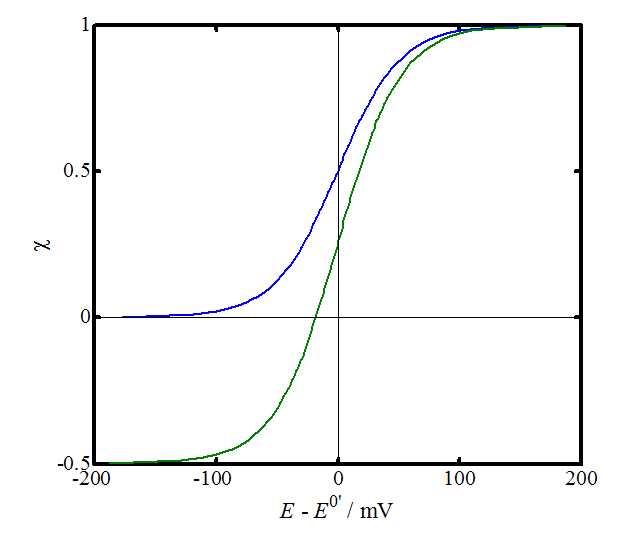 |
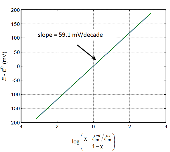 |
|---|
Figure 6.3 shows current-voltage curves with \( i_{\text{lim}}^{red}/{i_{\text{lim}}^{ox}}=0 \) or -0.5 and n = 1. The diffusion coefficients are usually rather close to one another, hence \( \xi^2 \approx1 \). Scaled current density \( \chi \) is defined as \( \chi=i/i_{\text{lim}}^{ox} \). Equation (6.21) provides a diagnostic criterion for a reversible electrode reaction: plotting the electrode potential as a function of the logarithm on the right-hand side of Equation (6.21), a straight line is obtained with a slope of 25.7/n mV, or on the log10 scale, 59.1/n mV per decade.
6.2.2 Quasi-reversible reaction
The derived equations above (6.15)-(6.19) are generally valid and can be used in Equation (6.12) to simulate current-voltage curves. Inserting Equation (6.17), for example, we find that
| \( \displaystyle \frac{i}{nF}=\frac{k_{ox}c_{\text{R}}^b-k_{red}c_{\text{O}}^b}{1+\frac{k_{ox}\delta}{D_{\text{R}}}+\frac{k_{red}\delta}{D_{\text{O}}}} \) | (6.22) |
|---|
In practice, the curves are preferably presented in terms of measurable quantities. The determination of the thickness of the DBL, \( \delta \), for example, is not unambiguous, as will be seen in Chapter 7.
Let us consider equilibrium again. Now, kred,eq cOb = kox,eq cRb because in the absence of electric current there is no concentration polarization, and surface concentrations are equal to bulk ones. At equilibrium, the rate of oxidation is equal to the rate of the reduction; they are not zero but the equilibrium is a dynamic process where the net reaction rate is zero. The Nernst equation is valid at equilibrium:
| \( \displaystyle\frac{c_{\text{O}}^b}{c_{\text{R}}^b}=e^{nf(E_{eq}-E^{0'})} \) | (6.23) |
|---|
Inserting the above equation into the expression of kred in Equation (6.10), we find that
| \( \displaystyle k_{red,eq}=k^0\left(\frac{c_{\text{O}}^b}{c_{\text{R}}^b}\right)^{\alpha-1} \) | (6.24) |
|---|
Exchange current density, i0, is defined as the inherent rate of oxidation or reduction at equilibrium:
\(\displaystyle i_0=nFk_{red,eq}c_{\text{O}}^b=nFk^0 c_{\text{O}}^b\left(\frac{c_{\text{O}}^b}{c_{\text{R}}^b}\right)^{\alpha-1}=nFk^0\left(c_{\text{O}}^b\right)^{\alpha}\left(c_{\text{R}}^b\right)^{1-\alpha} \) |
(6.25) |
|---|
Exchange current density is the measure of the rate of an electrode reaction, i.e. of its reversibility. A good reference electrode, such as Ag/AgCl has an exchange current as high as 10 A/cm2. Such an electrode is ideally non-polarizable, as discussed in Chapter 1.
The definition of overpotential is \( \eta=E-E_{eq} \). Hence, \( E-E^{0'}=E-E_{eq}+E_{eq}-E^{0'}= \eta+E_{eq}-E^{0'} \). The current-overpotential equation can be derived by applying Equation (6.23) to the last equality:
| \( \displaystyle\frac{i}{nF}=c_{\text{R}}^sk^0e^{\alpha nf\eta}\left(\frac{c_{\text{O}}^b}{c_{\text{R}}^b}\right)^{\alpha}-c_{\text{O}}^sk^0e^{(\alpha-1)nf\eta}\left(\frac{c_{\text{O}}^b}{c_{\text{R}}^b}\right)^{\alpha-1}=k^0(c_{\text{O}}^b)^{\alpha}(c_{\text{R}}^b)^{1-\alpha}\left[\frac{c_{\text{R}}^s}{c_{\text{R}}^b}e^{\alpha nf\eta}-\frac{c_{\text{O}}^s}{c_{\text{O}}^b}e^{(\alpha-1) nf\eta}\right] \) | (6.26) |
|---|
\( \displaystyle\frac{i}{i_0}=\frac{c_{\text{R}}^s}{c_{\text{R}}^b}e^{\alpha nf\eta}-\frac{c_{\text{O}}^s}{c_{\text{O}}^b}e^{(\alpha-1) nf\eta} \) |
(6.27) |
|---|
If the solution is stirred effectively or the current is less than 10% of the limiting current, the concentration polarization can be ignored, and the Butler-Volmer equation is obtained*:
| \( \displaystyle\frac{i}{i_0}=e^{\alpha nf\eta}-e^{(\alpha-1) nf\eta} \) | (6.28) |
|---|
The above equation is traditionally analyzed at limiting values of overpotential. At low overpotentials it can be linearized, giving
| \( \displaystyle i \approx i_0\frac{nF}{RT} \eta \Rightarrow \eta=\frac{RT}{nFi_0}i \) | (6.29) |
|---|
The unit of the group of variables RT/(nFi0) is \( \Omega \text{cm}^2 \); it is known as the charge transfer resistance, Rct.
At high positive overpotentials, only the anodic term of Equation (6.28) is significant. Hence
| \(\displaystyle \eta=-\frac{RT}{\alpha nF}\text{ln}i_0+\frac{RT}{\alpha nF}\text{ln}i \) |
(6.30) |
|---|
Accordingly, at high negative overpotentials only the cathodic term is significant:
| \( \displaystyle\eta=-\frac{RT}{(1-\alpha)nF}\text{ln}i_0+\frac{RT}{(\alpha-1)nF}\text{ln}|i| \) | (6.31) |
|---|
Equations (6.30) and (6.31) are called Tafel equations. The graphs of ln| i | vs. \( \eta \) are linear, and their extrapolation to zero overpotential gives the value of i0. This kind of a graph is called a Tafel plot. The original Tafel equation was empirical and written as
| \( \displaystyle\eta=a+b\log i \) | (6.32) |
|---|
where a and b were experimental constants; b is known as the Tafel slope. Comparing Equations (6.31) and (6.32), the cathodic Tafel slope is†
| \(\displaystyle b=\frac{2.303RT}{(\alpha-1)nF} \) | (6.33) |
|---|
Very often n = 1 and \( \alpha \approx0.5 \), giving a typical Tafel slope of approximately 120 mV per current decade. If mass transfer to the electrode is inefficient, the linear range of the plot can be rather limited due to concentration polarization, making the determination of Tafel slopes difficult. Measurements are therefore most often carried out with a rotating disk electrode (see Chapter 7.2.1), which makes the explicit elimination of mass transfer possible.
In a complete current-overpotential curve, mass transfer is taken into account. Inserting Equations (6.19) into Equation (6.27) the following expression can be derived:
| \( \displaystyle\chi=\frac{e^{\alpha nf\eta}-e^{(\alpha-1) nf\eta}}{\chi_{\text{kin}}+e^{\alpha nf\eta}+\chi_{\text{lim}}e^{(\alpha-1) nf\eta}} \) ; \( \chi_{\text{kin}}=\frac{i_{\text{lim}}^{ox}}{i_0} \) ; \( \chi_{\text{lim}}=\frac{i_{\text{lim}}^{ox}}{i_{\text{lim}}^{red}} \) |
(6.34) |
|---|
\( \chi \) is defined similarly to Figure 6.3, \( \chi=i/{i_{\text{lim}}^{ox}} \).
Figure 6.4 presents simulated curves using Equation (6.34). It shows the effect of the exchange current density: the lower it is, i.e. the higher \( \chi_{\text{kin}} \) is, the wider the potential range where hardly any current flows (potential window). At the limit i0 → 0 an electrode is ideally polarizable and its i-h graph horizontal. As discussed earlier, an ideally non-polarizable electrode has a very high exchange current density and without mass transfer limitations, its \( i-\eta \) graph would be vertical. In Figure 6.4, the curve with \( \chi_{\text{kin}}=0.1 \) is already completely under mass transfer control because with values lower than that the shape of the curve no longer changes.
An ideally non-polarizable electrode naturally cannot exist because solvent decomposes at high overpotentials. A mercury electrode is closest to an ideally polarizable electrode because the overpotential of hydrogen evolution (see paragraph 6.5.2) on mercury is very high, expanding the potential window over 2 V. Immiscible water-organic interfaces are also polarizable, although the potential window usually remains less than 1 V.
Figure 6.4. Simulated i-\( \eta \) curves with \( \chi \)kin = 0.1 -104, \( \alpha \) = 0.5, n = 1 or 2 and \( \chi \)lim = 2.
* The theory presented in this chapter is commonly called the Butler-Volmer theory and Equation (6.12) the Butler-Volmer equation, although it originally meant Equation (6.28).
† In an old polarographic convention, cathodic current was positive and, therefore, the current has no sign.
6.3. Overpotentials
We have already introduced the term overpotential* and defined this as the deviation from the equilibrium potential, \( \eta=E-E_{eq} \). In electrochemical literature, it is customary to split overpotential into activation (or charge transfer) and concentration overpotentials. If an electrode reaction were reversible, i.e. infinitely rapid (ideally non-polarizable electrode) and mass transfer were also infinitely rapid, the electrode potential would stay at its thermodynamic equilibrium value as determined by the Nernst equation, and no overpotential would exist. Overpotential means that the higher the current we are drawing out of an electrochemical cell, the higher the voltage needed above its thermodynamic cell voltage. In the case of a battery, overpotential means that when current is flowing we cannot utilize its full thermodynamic voltage (terminal voltage), it is instead lowered by the amount of overpotentials.
Tafel equations actually define the activation overpotential \( \eta_a \). Let’s write, for example, Equation (6.30) as
| \(\displaystyle \eta_a=\frac{RT}{\alpha nF}\text{ln}\frac{i}{i_0} \) | (6.35) |
|---|
which shows that the lower i0 is, the higher \( \eta_a \) is. We found earlier that current with \( \chi \)kin = 0.1 is under mass transfer control; hence it represents pure concentration overpotential. Subtracting the overpotential of this curve from the rest of the curves in Figure 6.4, we obtain the\( i-\eta_a \) curves in Figure 6.5, in other words the activation overpotential is the deviation from the y axis, depending on the current.
The origin of the concentration overpotential is in concentration polarization. Since the surface concentration is lower than the bulk concentration, a higher voltage is needed to draw current out of the cell. Equation (6.27) can be rewritten in the following form:
| \( \displaystyle\frac{i}{i_0}=\text{exp}\left[\alpha nf\eta_a+\text{ln}\frac{c_{\text{R}}^s}{c_{\text{R}}^b}\right]-\text{exp}\left[(\alpha-1)nf\eta_a+\text{ln}\frac{c_{\text{O}}^s}{c_{\text{O}}^b}\right] \) | (6.36) |
|---|
that shows that the concentration overpotential, \( \eta_c \), is of the form
| \( \displaystyle\eta_c=\frac{RT}{nF}\text{ln}\frac{c^s}{c^b} \) | (6.37) |
|---|
Figure 6.5. Current-overpotential curves after subtracting for the concentration overpotential. \( \chi \)kin = 10 - 104 , \( \alpha \) = 0.5, n = 1 or 2.
If an electrode reaction is accompanied by homogeneous reactions (e.g. EC/CE mechanism) they make their contribution, known as the reaction overpotential. When there is a phase formation on the electrode, such as the deposition of metal, the formation and growth of the phase nuclei cause the nucleation overpotential that depends on surface chemical issues, including the geometry of the nuclei. Reaction and nucleation overpotentials are not addressed in this book in a closer detail.
It is necessary to remember that in addition to overpotentials an electrochemical cell always has ohmic losses due to the limited conductivity of electrolytes (see Chapter 3 and 4).
6.4. The effect of electric double layer
An electric double layer (EDL, see Chapter 5) has an effect on an electrode reaction through two factors. First, in order for an electron transfer to occur, the species involved in the reaction must reside so close to the surface of the electrode that an electron can be tunneled between the species and the electrode. In the previous chapter it was shown that at this close vicinity of the surface, the concentration of a charged species is different from its bulk concentration according to the Boltzmann distribution:
| \( \displaystyle c_i(x_2)=c_i^be^{-z_if\phi_2} \) |
(6.38) |
|---|
If mass transfer needs to be taken into account, the bulk concentration is replaced by the surface concentration calculated from mass transfer equations.
Second, at the distance x2 from the electrode the driving force of electron transfer is not \( E-E^{0'} \) but \( E-\phi_2-E^{0'} \). Taking this into account, as well as Equation (6.38), the expression of kox, for example, becomes
| \( k_{ox}=k^0e^{\displaystyle -z_{\text{R}}f\phi_2}e^{\displaystyle\alpha nf(E-\phi_2-E^{0'})}=k^0e^{\displaystyle -(\alpha n+z_{\text{R}})f\phi_2}e^{\displaystyle\alpha nf(E-E^{0'})} \) | (6.39) |
|---|
The correction factor \( e^{-(\alpha n+z_{\text{R}})f\phi_2} \) is known as the Frumkin correction. If the calculation of \( \phi_2 \) is feasible, the actual k0 is denoted as kt0 (’t’ = true). The experimental value of k0, calculated from i0 for example, is therefore
| \( k^0=k_t^0e^{\displaystyle -(\alpha n+z_{\text{R}})f\phi_2} \) | (6.40) |
|---|
An analogous result is achieved for kred, taking into account that n = zO - zR.
Equation (6.38) can be derived from the equilibrium condition between the bulk solution and the electric double layer, \( \tilde{\mu}_i(x_2)=\tilde{\mu}_i^b \) , that is strictly speaking only valid in the absence of electric current. The formally correct method would be to integrate the Nernst-Planck equation (3.34) from the bulk (x = \( \delta \)) to the distance x2. The result of this procedure is known as the Levich correction:
| \( \displaystyle c_i(x_2)=e^{-z_if\phi_2}\left(c_i^b-\frac{i}{nFD_i} \int_{\delta}^{x_2}{e^{z_if\phi}dx}\right) \) | (6.41) |
|---|
Corrections to the EDL are usually not made because it would require the calculation of the potential profile at each electrode potential, which depends on the chosen microscopic model of the EDL. The calculation of the Frumkin correction is not common either, and experimental (yet apparent) values usually suffice perfectly well. Chapter 7 briefly looks at the effect of the EDL on electrochemical experiments in connection with respective techniques.
6.5. Electrochemical reaction mechanisms
Like all chemical reactions, electrochemical reactions may also consist of several consequtive reaction steps; parallel steps also occur. Reaction mechanisms can be studied with current-voltage curves and in particular with Tafel slopes. The reduction of copper provides a well-known example of a two-step reaction:
| Cu2+ + e- → Cu+ slow | (6.42) |
|---|
| Cu+ + e- → Cu fast | (6.43) |
|---|
The rate constant of the first step has been determined* as \( k_1^0=6.50 \times10^{-5} \text{ cm s}^{-1} \), and that of the second step \( k_2^0=0.139 \text{ cm s}^{-1} \). The second step has also been found to be reversible: the reverse zeroth order reaction rate constant is \( k_{-2}^0=1.88 \times10^{-7} \text {cm}^{-2} \text{s}^{-1} \). Copper is also famous for its disproportionation reaction
| 2 Cu+ → Cu2+ + Cu | (6.44) |
|---|
that has the equilibrium constant of \( 2.20 \times10^{-6} \). As this example shows, an electrochemical reaction can be quite complicated but, like in all reaction kinetics, one step may be rate-determining which simplifies the analysis greatly.
Since the reaction rate is proportional to the electric current, the reaction order, \( \nu_k \), of a species k in the reaction can be determined simply as
| \( \displaystyle\nu_k=\left(\frac{\partial\text{ln}i}{\partial\text{ln}c_k}\right) \) | (6.45) |
|---|
The determination of the reaction order can help in the solving of the reaction mechanism. If the reaction order of a species is zero, for example, it is not part of the electron transfer chain.
6.5.1 Tafel slopes of a two-step reaction
Let’s consider a reaction like that of copper, \(\ce{ R<=>O }\) \( +2\text{ e}^- \) , with the following notation:
| \(\ce{ R <=>[\ce{k_1}][\ce{k_{-1}}] X }\) \( +\text{ e}^- \) | (6.46) |
|---|
| \(\ce{ R <=>[\ce{k_2}][\ce{k_{-2}}] O }\) \( +\text{ e}^- \) | (6.47) |
|---|
The charge transfer coefficient and the formal potential of the first step (6.46) are \( \alpha \) and \( E_1^{0'} \) respectively, and those of the second step (6.47) \( \alpha_2 \) and \( E_2^{0'} \). In the stationary state the reaction rates of steps 1 and 2 are equal, hence d[X]/dt = 0. The total current density is the sum of the currents of the individual steps, i = i1 + i2, therefore i1 = i2 = (1/2)i. Since we are going to derive the Tafel slopes as a function of the rates of the individual reaction steps we consider the potential range where mass transfer is insignificant. Therefore, cR and cO assume their bulk values but the concentration of the intermediate X, cX, depends on the electrode potential. Furthermore, it is assumed that X is not desorbed from the electrode and transported away.
Now we are able to write down the reaction rates in a stationary state:
| \( \displaystyle\frac{1}{2}\frac{i}{F}=\frac{i_1}{F}=k_1^0(c_\text{R}e^{\alpha_1f(E-E^{0'}_1)}-c_\text{X}e^{(\alpha_1-1)f(E-E^{0'}_1)}) \) | (6.48) |
|---|
| \( \displaystyle\frac{1}{2}\frac{i}{F}=\frac{i_2}{F}=k_2^0(c_\text{R}e^{\alpha_2f(E-E^{0'}_2)}-c_\text{O}e^{(\alpha_2-1)f(E-E^{0'}_2)}) \) | (6.49) |
|---|
At equilibrium, the current is zero, i.e. the currents in both steps are zero. At the equilibrium potential, Eeq, the concentration of X is cX,eq. Analogously to Chapter 6.2.2, we can write down the exchange current densities of the reaction steps
| \( \displaystyle i_{0,1}=Fk_1^0(c_{\text{X,eq}})^{\alpha_1}(c_{\text{R}})^{1-\alpha_1} \) |
(6.50) |
|---|
| \( \displaystyle i_{0,2}=Fk_2^0(c_{\text{O}})^{\alpha_2}(c_{\text{X,eq}})^{1-\alpha_2} \) |
(6.51) |
|---|
Current-overpotential equations accordingly become
| \( \displaystyle\frac{i_1}{i_{1,0}}=e^{\alpha_1f\eta}-\left(\frac{c_{\text{X}}}{c_{\text{X,eq}}}\right)e^{(\alpha-1)f\eta} \) |
(6.52) |
|---|
| \( \displaystyle\frac{i_2}{i_{2,0}}=\left(\frac{c_{\text{X}}}{c_{\text{X,eq}}}\right)e^{\alpha_2f\eta}-e^{(\alpha_2-1)f\eta} \) | (6.53) |
|---|
Eliminating (cX/cX,eq) from the above equations, current density is obtained as \( i=2 \cdot i_1=2 \cdot i_2 \):
| \( \displaystyle i=\frac{2(e{^f\eta}-e^{-f\eta})}{(i_{1,0})^{-1}e^{(1-\alpha_1)f\eta}+(i_{2,0})^{-1}e^{-\alpha_2f\eta}} \) | (6.54) |
|---|
When \( f\eta \) » 0, the terms with negative exponential become insignificant, and the anodic Tafel equation is found to be
| \( \displaystyle\eta=\frac{2.303RT}{\alpha_1F}\text{log}(i)-\frac{2.303RT}{\alpha_1F}\text{log}(2i_{1,0}) \) | (6.55) |
|---|
Analogously, when \( f\eta \) « 0, the cathodic Tafel equation is
| \( \displaystyle\eta=\frac{2.303RT}{(\alpha_2-1)F}\text{log}(-i)+\frac{2.303RT}{(1-\alpha_2)F}\text{log}(2i_{2,0}) \) |
(6.56) |
|---|
At sufficiently large overpotentials, the Tafel slopes correspond to one electron transfer, ±118 mV/decade (if \( \alpha_1=\alpha_2=0.5 \)). Extrapolating the Tafel slopes to zero overpotential, i1,0 and i2,0 can be determined. Hence if the intercepts at the current axis are not equal a multi-step mechanism is expected. It is also worth noting that \( \alpha_1+\alpha_2 \) is not necessarily equal to unity.
From Equation (6.54) it is easy to see the effect of the rate-determining step on the Tafel slopes. If i1,0 » i2,0 so the first term in the denominator can be neglected, the anodic Tafel slope is \( \frac{2.303RT}{(1+\alpha_2)F} \), ca. 40 mV/decade if \( \alpha_2=0.5 \). This can be seen in the first curve of Figure 6.6 in the range -2 < log| i/i0,1| < 1; the cathodic Tafel slope follows Equation (6.56). Similarly, if i1,0 « i2,0 the anodic Tafel slope follows Equation (6.55), and the cathodic slope is \( -\frac{2.303RT}{(2-\alpha_1)F} \), the last curve in Figure 6.6 in the range 1 < log| i / i0,1| < 4. At very high overpotentials, Equations (6.55) and (6.56) are valid, as Figure 6.6 also proves. In the case of copper, i1,0 » i2,0, giving the current-overpotential equation
| \( \displaystyle i=2i_{2,0}(e^{(1+\alpha_2)f\eta}-e^{(\alpha_2-1)f\eta}) \) | (6.57) |
|---|
The anodic Tafel slope is approximately 40 mV/decade and the cathodic slope approximately 120 mV/decade, which is experimentally found to be correct.
Another example is the reaction
| Mn4+ + e- → Mn3+ | (6.58) |
|---|
At first glance, the reaction appears to be a simple one-electron transfer, but the concentration of Mn4+ has no effect on current, i.e. its reaction order is zero while the reaction order of Mn3+ is one. The mechanism that explains these results is
| Mn3+ + e- \(\ce{ <=> }\) Mn2+ k1, k-1 | (6.59) |
|---|
| Mn4+ + Mn2+ \(\ce{ <=> }\) 2 Mn3+ k2, k-2 | (6.60) |
|---|
| Mn4+ + e- \(\ce{ <=> }\) Mn3+ | (6.58) |
|---|
Let’s denote [Mn2+] = c1, [Mn3+]
= c2 and [Mn4+] = c3. In
the cathodic potential range, the inverse reaction of (6.59) can be neglected. Making
the steady-state approximation of Mn2+ which does not appear in the
net reaction
| \( \displaystyle\frac{dc_1}{dt}=k_1c_2-k_2c_1c_3+k_{-2}c_2^2=0 \Rightarrow \nu=-\frac{dc_3}{dt}=k_2c_1c_3-k_{-2}c_2^2=k_1c_2 \) | (6.61) |
|---|
Equation (6.61) confirms that the reaction is of the first order with respect to Mn3+ and of the zeroth order with respect to Mn4+. Since the disproportionation reaction (6.60) does not include electron transfer, the concentration of Mn4+ does not contribute to electric current; the reaction therefore represents an EC mechanism.
If reaction (6.60) were rate-determining, Mn2+ would accumulate to such a large extent that the inverse reaction of (6.59) should also be taken into account. In general, reactions preceding the rate-determining step stay at equilibrium and, therefore, c1 = K1c2 where K1 would be the equilibrium constant of reaction (6.59). This would convert Equation (6.61) into the form of (k-2 = 0)
| \( \displaystyle\nu=-\frac{dc_3}{dt}=k_2K_1c_2c_3 \) | (6.62) |
|---|
The net reaction would therefore be of the first order with respect to both Mn3+ and Mn4+. As K1 is a function of the electrode potential† according to the Nernst equation and k2 is independent of potential, the Tafel slope would be 59 mV/decade.
Finally, let’s compare the following mechanisms semi-qualitatively:
| A +
e-\(\ce{ <=>[\ce{k_1}] }\) B
+ e- \(\ce{ ->[\ce{k_2}] }\) C |
(6.63) |
|---|
| \( \displaystyle\begin{cases}\text{A}+\text{e}^- \rightarrow \text{B}\text{, }k_1 \\\text{A}+\text{e}^- \rightarrow \text{C}\text{, }k_2\end{cases} \) | (6.64) |
|---|
If the first step of the consequtive reaction mechanism (6.63) is rate-determining, as soon as B is formed, it reacts further to C. Since both steps include electron transfer, the total current is i = 2·i1, but the Tafel slope is determined from the first step. If the second step is rate-determining, i = 2·i2 and the Tafel slope is \( -\frac{2.303RT}{(2-\alpha_2)F} \) because
| \( -\displaystyle\frac{i_2}{F}=[B]k_2^0e^{(\alpha_2-1)f(E-E_2^{0'})}=[A]e^{-f(E-E_1^{0'})}k_2^0e^{(\alpha_2-1)f(E-E_2^{0'})}=[A]e^{-f(E_2^{0'}-E_1^{0'})}k_2^0e^{-f(2-\alpha_2)(E-E_2^{0'})}=\text{constant} \cdot e^{f(\alpha_2-2)(E-E_2^{0'})} \) | (6.65) |
|---|
The analysis of parallel reactions (6.64) is easier: i = i1 + i2 and the Tafel slope is determined by the faster reaction. If \( \alpha_1 \) and \( \alpha_2 \) are significantly different, the Tafel slope may vary because the rates of the individual reactions vary at a different pace as a function of the electrode potential. In Figure 6.7, at low electrode potentials the first reaction with higher exchange current density i0,1 and \( \alpha_1=0.3 \) controls current, but at higher electrode potentials the other reaction with lower exchange current density i0,2 and \( \alpha_2=0.7 \) takes control because the exponential function overcomes the difference in exchange current densities.
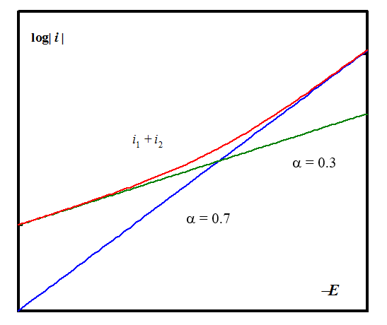
6.5.2 Hydrogen evolution
Hydrogen evolution is probably the most studied electrochemical reaction due to its immense industrial significance. In the electrolytic production of metals, for example, hydrogen evolution defines the upper limit of the cathodic overpotential that can be used; this issue was discussed in Chapter 4 in connection with Pourbaix diagrams. Splitting water into hydrogen and oxygen in an electrolyzer is another application that may be particularly important in hydrogen economy in the future, see Chapter XX. Furthermore, the inverse reaction of hydrogen evolution, the catalytic dissociation of hydrogen to protons and electrons, is the core reaction in the hydrogen fuel cell.
The rate of hydrogen evolution very much depends on the electrode material, because the reaction includes an adsorption step as described below. The ability of a metal to facilitate hydrogen evolution is illustrated in the volcano plot, Figure 6.8.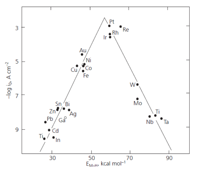
Figure 6.8. Volcano plot: The dependence of the exchange current density of the hydrogen evolution reaction on the adsorption enthalpy of hydrogen. From: Holton et al., Platinum Metals Review, 57 (2013) 259-271 (with publisher’s permission).
The volcano plot is represented in various ways in the literature, but its interpretation is the same. If the adsorption of hydrogen on a metal is relatively weak – low adsorption enthalpies – hydrogen remains on the surface for such a short time that the reaction cannot proceed to a significant extent. If hydrogen is tightly bound to the surface – high adsorption enthalpies – the reaction does not proceed on from the adsorption step. The optimal strength of the metal-hydrogen bond is reached with the platinum group metals, which are the best catalysts for hydrogen evolution. The bond energy of H2 is 4.52 eV corresponding to approximately 100 kcal/mol. The adsorption step thus lowers the energy barrier by approximately 60% for these metals. Since they are rather expensive and not abundantly available, new catalyst materials are being sought to help achieve hydrogen economy. Promising results have been obtained with modified carbon nanotubes, for example‡.
In the previous chapter, two salient methods for determining a reaction mechanism were introduced: the steady-state approximation for short-lived reaction intermediates and the analysis of the rate-determining step. In hydrogen evolution, the adsorption step must be taken into account.
The net reaction of hydrogen evolution in an
acidic solution is
| 2 H3O+ + 2 e- \(\ce{ <=> }\) H2 + 2 H2O | (6.66) |
|---|
The standard potential of reaction (6.66) is E0 ≡ 0.00 V according to the IUPAC convention (NHE = normal hydrogen electrode). In an alkaline solution the reaction is
| 2 H2O + 2 e- \(\ce{ <=> }\) H2 + 2 OH- E0 = -0.828 V (NHE) | (6.67) |
|---|
In a neutral solution, the inverse reaction of (6.66) dominates on the anode and reaction (6.67) on the cathode. The electrode potentials change by 59 mV/pH unit. It is also necessary to realize that the pH of the solution may change as a result of the reactions.
Hydrogen evolution is traditionally analyzed via the following elementary reactions:
1. Volmer reactions
| H3O+ + e- \(\ce{ <=> }\) H* + H2O acidic solution | (6.68a) |
| H2O + e- \(\ce{ <=> }\) H* + OH- neutral/alkaline
solution |
(6.68b) |
|---|
2. Heyrovský reactions
| H* + H3O+ + e- \(\ce{->} \) H2(g) + H2O acidic solution | (6.69a) |
| H* + H2O + e- \(\ce{ -> }\) H2(g) + OH- neutral/alkaline solution |
(6.69b) |
|---|
3. Tafel reaction
| 2 H* \(\ce{ -> }\) H2(g) | (6.70) |
|---|
H* denotes an adsorbed hydrogen atom. The electrode material has a large impact on the contributions of these elementary reactions to the net reaction.
6.5.2.1 Volmer-Heyrovský mechanism:
Let us first consider the Volmer-Heyrovský mechanism in an acidic solution. Since the standard potentials of the elementary reactions, E0, are unknown, we cannot use the standard rate constant, k0, but each reaction has its own rate constant in the rate equation.
| H3O+ + e- \(\ce{ <=>[\ce{\nu_1}][\ce{\nu_{-1}}] }\) H* + H2O | |
| H* + H3O+ + e− \(\ce{ ->[\ce{\nu_2}] }\) H2(g) + H2O |
|
| \( \nu_1=k_1[\text{H}^+](1-\theta)e^{(\alpha-1)fE} \) |
|
| \( \nu_{-1}=k_{-1}^0\theta e^{\alpha fE} \) |
(6.71) |
|---|
where E is the electrode potential on an arbitrary scale and \( \theta \) is the surface coverage of an adsorbed hydrogen atom. Writing these in terms of the overpotential \( \eta(E=E_{eq}+E-E_{eq}=E_{eq}+\eta) \) Equations (6.71) take on the forms
| \( \nu_1=k_1[\text{H}^+](1-\theta)e^{(\alpha-1)f\eta} \) |
|
| \( \nu_{-1}=k_{-1}^0\theta e^{\alpha f\eta} \) |
(6.72) |
|---|
Note that the cathodic Volmer reactions is of the first order with respect to the proton concentration, but the anodic reaction of the 0th order. This also tells us that adsorption can only take place on the non-occupied surface of an electrode that is described with 1 - \( \theta \). Accordingly, the rate of the Heyrovský reaction becomes
| \( \displaystyle\nu_2=k_2^0[\text{H}^+]\theta e^{(\alpha-1)fE}=k_2[\text{H}^+]\theta e^{(\alpha-1)f\eta} \) |
(6.73) |
|---|
The transfer coefficient \( \alpha \) is traditionally assumed to be equal in the both reactions. The steady-state approximation is made for the adsorbed hydrogen: \( d\theta/dt=\nu_1-\nu_{-1}-\nu_2=0 \):
| \( \displaystyle k_1[\text{H}^+](1-\theta)e^{(\alpha-1)f\eta}-k_{-1}\theta e^{\alpha f\eta}-k_2[\text{H}^+]\theta e^{(\alpha-1)f\eta}=0 \) |
(6.74) |
|---|
Solving \( \theta \) from Equation (6.74) gives:
| \( \displaystyle\theta=\frac{k_1[\text{H}^+]}{(k_1+k_2)[\text{H}^+]+k_{-1}e^{f\eta}} \) | (6.75) |
|---|
Two limiting cases can be studied from Equation (6.75): a) \( \theta \approx0 \)and b) \( \theta \approx1 \). Case a) is reached with the condition k-1 » k1, k2. Note that \( \eta<0 \) because hydrogen is evolved. At low cathodic overpotentials:
| \( \displaystyle\theta \approx\frac{k_1[\text{H}^+]}{k_{-1}} e^{-f\eta}=K_1[\text{H}^+]e^{-f\eta} \) | (6.76) |
|---|
where K1 is the equilibrium constant of the Volmer reaction. Because at steady-state the rate of the Volmer reaction must be equal to the rate of the Heyrovský reaction, v1 - v-1 = v2. One electron is transferred in the both steps. Hence, inserting Equation (6.76) into Equation (6.73) the following is obtained:
| \( \displaystyle\frac{i}{F}=2\nu_2=2k_2K_1[\text{H}^+]^2e^{(\alpha-2)f\eta} \) | (6.77) |
|---|
| \( \displaystyle\frac{\partial\text{ ln }i}{\partial\eta}=(\alpha-2)f \) or \( \frac{\partial\eta}{\partial\text{ log }i}=2.303\frac{\partial\eta}{\partial\text{ ln }i}=2.303\frac{1}{\alpha-2}\frac{RT}{F} \) |
(6.78) |
|---|
If \( \alpha \) = 0.5 the Tafel slope is capproximately -40 mV, which provides a diagnostic criterion for the mechanism. Another criterion comes from the reaction order:
| \( \displaystyle \frac{\partial\text{ ln }i}{\partial\text{ ln }[\text{H}^+]}=2 \) | (6.79) |
|---|
Current therefore increases 100-fold when pH decreases one unit.
Case b) is reached at high cathodic overpotentials if k1 » k-1, k2. Current is now
| \( \displaystyle\frac{i}{F}=2k_2[\text{H}^+]e^{(\alpha-1)f\eta} \) because \( \theta \approx1 \) |
(6.80) |
|---|
| \( \displaystyle\frac{\eta}{\partial\text{ log }i}=2.303\frac{1}{\alpha-1}\frac{RT}{F} \) | (6.81) |
|---|
| \( \displaystyle\frac{\partial\text{ ln }i}{\partial [\text{H}^+]}=1 \) | (6.82) |
|---|
The Tafel slope therefore is approximately -120 mV if \( \alpha=0.5 \), and the reaction order with respect to the proton concentration is unity, i.e. current increases 10-fold when pH decreases one unit. The graphs of Equations (6.73) and (6.75) are shown below.
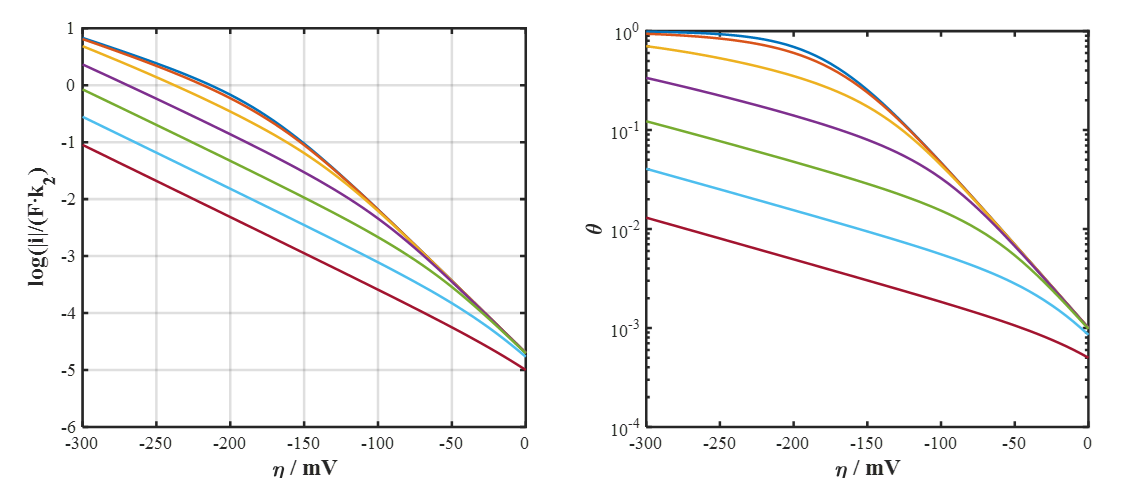
Figure 6.9. Scaled current density (left) and surface coverage (right) as a function of overpotential according to the Volmer-Heyrovský mechanism. K1 = 0.1 and k2/k−1 = 10−3, 10−2, 0.1, 1, 10 and 100 from top to bottom, pH = 2. Increasing K1 shifts the point where Tafel slope changes from 40 mV to 120 mV towards lower cathodic overpotentials (to the right).
6.5.2.2 Volmer-Tafel mechanism:
The analysis of the Volmer reactions remains the same, and the rate of the Tafel reaction can analogously be written as:
| 2 H* \(\ce{ ->[\ce{\nu_3}] }\) H2(g) | |
| \( \nu_3=-\frac{1}{2}\frac{d\theta}{dt}=k_3\theta^2 \) |
(6.83) |
|---|
The steady-state approximation is now d\( \theta \)/dt = v1 - v-1 - 2v3 = 0:
| \( k_1[\text{H}^+](1-\theta)e^{(\alpha-1)f\eta}-k_{-1}\theta e^{\alpha f \eta}-2k_3\theta^2=0 \) |
(6.84) |
|---|
Solving for the surface coverage \( \theta \) would require the solution of the second order algebraic equation, which would not be very demonstrative. We therefore look again at the limiting cases \( \theta \approx0 \) and \( \theta \approx1 \).
If \( \theta \approx0 \), the second order term of Equation (6.84) vanishes, and from the remaining equation
| \( \displaystyle\theta \approx \frac{k_1[\text{H}^+]}{k_1[\text{H}^+]+k_{-1}e^{f\eta}} \) |
(6.85) |
|---|
In order to have the surface coverage close to zero, it must be valid that k-1 » k1. Thus,
| \( \displaystyle\theta \approx\frac{k_1[\text{H}^+]}{k_{-1}} e^{-f\eta}=K_1[\text{H}^+]e^{-f\eta} \) | (6.86) |
|---|
| \( \displaystyle\frac{i}{F}=2k_3K_1^2[\text{H}^+]^2e^{-2f\eta} \) | (6.87) |
|---|
Equation (6.87) shows that the reaction is of the second order with respect to the proton concentration (see Eq. (6.79)). The Tafel slope is now
| \( \displaystyle\frac{\partial\eta}{\partial\text{ log }i}=2.303\frac{RT}{F} \approx30\text{ mV} \) | (6.88) |
|---|
If the surface coverage \( \theta \) approaches unity, it is obtained directly from Equation (6.84) that
| \( \displaystyle\frac{i}{F}=k_3=\text{constant} \) | (6.89) |
|---|
This condition is fulfilled if k1 » k-1, k3. The current would in this case be kinetically limited and not dependent on overpotential or pH.
A full simulation to Equations (6.83) and (6.84) is shown in Figure 6.10.
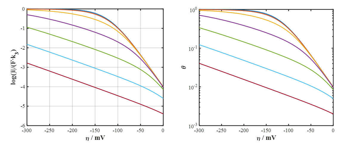
Figure 6.10. Scaled current density (left) and surface coverage (right) as a function of overpotential according to the Volmer-Tafel mechanism. K1 = 1 and k3/k−1 = 10−3, 10−2, 0.1, 1, 10 and 100 from top to bottom, pH = 2. Increasing K1 shifts the point where Tafel slope changes from 30 mV to infinity towards lower cathodic overpotentials (to the right).
6.5.2.3 Equilibrium and the rate-determining step
If the second step, be it of the Heyrovský or Tafel reaction, is rate-determining, the first step remains at equilibrium at all times. Writing this in calculus, v1 = v-1, and using Equation (6.72), an electrochemical Langmuir isotherm is obtained:
| \( \displaystyle\frac{\theta}{1-\theta}=K_1[\text{H}^+]e^{-f\eta} \Leftrightarrow \theta=\frac{K_1[\text{H}^+]e^{-f\eta}}{1+K_1[\text{H}^+]e^{-f\eta}} \) | (6.90) |
|---|
The rate of the net reaction depends on the prevailing mechanism (Heyrovský or Tafel). It is easy to show that the steady-state approximation used above, d\( \theta \)/dt = 0, is valid only when the second step is rate-determining. At high cathodic overpotentials, the surface coverage approaches unity, and at low overpotentials it approaches zero.
* S. Krzewska, Electrochim. Acta, 42 (1997) 3531. (acidic solution)
† \( K_1=\text{exp}[-f(E-E_1^{0'})] \)
‡ Tavakkoli et al. Angewandte Chemie, 54 (2015) 4535-4538.
6.6. Oxygen reduction
...
6.7. Corrosion
In corrosion, two simultaneous reactions are taking place on a metal surface so that the anodic current is equal but opposite in sign to the cathodic current, Ia = |Ic| = Icorr, the corrosion current. Although the net current in corrosion is zero the exchange current can be quite high. Since the anodic and cathodic reactions are not directly connected to one another, their potential dependence and charge transfer coefficients (\( \alpha \)) are mutually independent. The metal surface is settled at a corrosion potential Ecorr where the net current is zero. The corrosion potential does not represent a true thermodynamic equilibrium because reactions are proceeding, and it can also vary during the corrosion process as the surface areas involved in the anodic and cathodic reactions change as corrosion progresses.
The dissolution of a metal can be written as an anodic reaction
| M \(\ce{ -> }\) Mn+ + ne- | (6.105) |
|---|
A cathodic reaction that
balances the electric charge depends on the pH of the solution. In a neutral or acidic
solution they are
| O2 + 4 H+ + 4 e– \(\ce{ \bond{->} }\) 2 H2O (neutral) | (6.106a) |
| 2 H+ + 2
e– \(\ce{ \bond{->} }\)
H2 (acidic) |
(6.106b) |
|---|
In an alkaline solution, the following reactions are possible:
| O2 + 2 H2O + 4 e– \(\ce{ \bond{->} }\) 4 OH– | (6.107a) |
| 2 H2O + 2 e– \(\ce{ \bond{->} }\) H2 + 2 OH– | (6.107b) |
|---|
Corrosion is often accompanied by the formation of an oxide film on the metal surface. Such a film is a poor charge carrier (semi-conductor) and passivates the surface, preventing further corrosion. Several metals such as various types of steel, chromium, aluminium, zirkonium, tantalum and titanium form a passivating film, the properties of which determine their corrosion resistance. Copper forms a stable Cu2O film or patina that gives the characteristic beautiful color to copper surfaces.
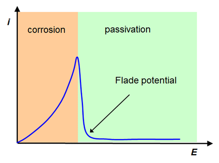
|
Table 6.1. Passivation potential of selected metals, EF0 (potential with the maksimum corrosion current); pH = 0, T = 298 K. (J.O’M. Bockris and A.K.N. Reddy, Modern Electrochemistry, Plenum Press, New York 1970, s. 1317.) |
|
|
Metal |
EF0 / V vs. NHE |
|
Au |
+1.36 |
|
Pt |
+0.91 |
|
Fe |
+0.58 |
|
Ag |
+0.40 |
|
Ni |
+0.36 |
|
Cr |
-0.22 |
|
Ti |
-0.24 |
A great deal of corrosion studies concern iron (steel) due to its immense industrial significance. A qualitative current-voltage curve of steel in Figure 6.11 shows the passivation of the film and the termination of corrosion at potentials which are positive to the Flade potential.
The Flade potential is a
linear function of pH and often of the form
| \( E_{\text{F}}=E_{\text{F}}^0-\text{pH} \times 0.059{\text{ V}} \) | (6.108) |
|---|
One of the oldest and
best known results about the corrosion of iron is that it dissolves readily in
diluted nitric acid but not in concentrated nitric acid. Iron dissolution is:
| Fe → Fe2+ + 2 e- | (6.109) |
|---|
The cathodic reaction is
the reduction of nitrate:
| NO3- + 2 H+ + 2 e- → NO2 + H2O | (6.110) |
|---|
Looking at reaction (6.110), the reaction rate should increase at a lower pH contrary to Equation (6.108). Obviously the corrosion of iron is determined by kinetics, and a purely thermodynamic analysis based on, for example, Bourbaix diagrams (Chapter 4) does not give the real picture. Based on Figure 6.11, it can be concluded that in very acidic conditions the corrosion potential of iron is on the negative side of the Flade potential and in moderately acidic solutions on its positive side. The impedance analysis of corrosion is discussed in Chapter 9.
6.8. Marcus theory
In 1992, Rudolf Marcus received the Nobel Prize in Chemistry for the theory of electron transfer that is commonly known as the Marcus theory. Its predecessors are the studies by Levich [1] and Dogonadze [2] about the reorganization of solvent molecules during a redox reaction. The approach taken by Marcus is based on statistical mechanics, considering the configurations of all molecules participating in the reaction. Each molecule is described as a harmonic oscillator, with an energy that depends in a parabolic manner on the deflection from its equilibrium position. As there are several molecules, each having several modes of vibration, a multi-dimensional energy space is obtained that is very difficult to visualize. We simplify the situation to the two-dimensional Figure 6.12. This approach [3] is closer to the models of Levich and Dogonadze, but is simpler than the accurate treatise by Marcus yet gives the same results.
On the right of Figure 6.11 the free energy profile of the oxidized species ’ox’ is seen. At configuration xox its free energy is Gox. Similarly, the reduced species’red’ has its energy profile on the left: its free energy at configuration xred is Gred. In this simple model, the reaction coordinate can be interpreted as the stretch of the molecular bond from its equilibrium length. The energy profiles intersect at configuration xc, where an electron is transferred from red to ox in an adiabatic process.
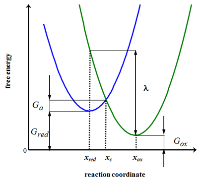
Let’s calculate the abscissa of the intersection of the parabolas, xc:
| \( \displaystyle G_{ox}^c=G_{ox}+\frac{1}{2}h\nu(c_x-x_{ox})^2=G_{red}+\frac{1}{2}h\nu(c_x-x_{red})^2=G_{red}^c \) | (6.111) |
|---|
| \( \displaystyle x_c=\frac{1}{2}(x_{ox}-x_{red})+\frac{\Delta G}{h\nu(x_{ox}-x_{red})} \) ; \( \Delta G=G_{ox}-G_{red} \) |
(6.112) |
|---|
Note that \( \Delta G<0 \). The factor \( h\nu \) is the energy of the fundamental vibration of a harmonic oscillator that is obtained from its quantum mechanical solution; h is the Planck constant, 6.626×10⁻³⁴ Js and \( \nu \) is the vibration frequency (s–1). Inserting the expression of xc into that of Gred, the height of the energy barrier (activation energy) is found to be
| \( \displaystyle\Delta G_a=G_{red}^c-G_{red}=\frac{(\lambda+\Delta G)^2}{4\lambda} \) |
(6.113) |
|---|
| \( \displaystyle\lambda=\frac{1}{2}h\nu(x_{ox}-x_{red})^2 \) | (6.114) |
|---|
The quantity \( \lambda \) is known as the reorganization energy, because it represents the energy change when moving along either of the parabolas between the points xred and xox, i.e. the change in the molecular configuration without electron transfer. It is always a positive quantity.
The rate constant of the reaction is expressed via the theory of activated complexes (absolute rate theory):
| \( \displaystyle k=\frac{k_{\text{B}}T}{h}\kappa e^{-\Delta G_a/RT}=k'e^{-\Delta G_a/RT} \) | (6.115) |
|---|
kB is the Boltzmann constant (1.38×10⁻²³ J K–1) and \( \kappa \) is what is known as transmission coefficient, which is unity for an adiabatic reaction. When the electrode potential is changed, this changes \( \Delta G \) as discussed earlier in this chapter. The charge transfer coefficient \( \alpha \) is therefore found to be
| \( \displaystyle\alpha=\frac{RT}{F}\frac{\partial\text{ln }k}{\partial E}=-\frac{1}{F}\frac{\partial\Delta G_a}{\partial E}=-\frac{1}{2F}\left(1+\frac{\Delta G}{\lambda}\right)\frac{\partial\Delta G}{\partial E}=\frac{1}{2}\left(1+\frac{\Delta G}{\lambda}\right) \) | (6.116) |
|---|
because
| \( \displaystyle\Delta G =-F(E-E^0) \) | (6.117) |
|---|
Thus, if \( \lambda \gg\Delta G \), \( \alpha \approx0.5 \), as is usually found to be the case in experiments in the vicinity of an equilibrium potential. When \( \Delta G \) is increased, the intercept xc approaches the point xred whence\( \Delta G=-\lambda \), Ga = 0 and \( \alpha=0 \). When the intercept xc moves to the left side of xred, Ga starts to increase again, i.e. the reaction rate begins to decrease. This range of potentials is known as the inverted region; its existence was not verified until 1990s. If \( \Delta G>0 \), i.e. the parabola of the species ox is raised with respect to that of the species red, the activation energy increases and \( \alpha \) ultimately approaches unity (\( \Delta G=\lambda \)).
The discussion above covers the reaction ’from left to right’. Considering the inverse reaction ‘from right to left’, it is seen from Figure 6.12 that the activation energy is higher by the amount of \( -\Delta G \). From Equation (6.113) we therefore see that
| \( \displaystyle\Delta G_a'=\Delta G_a-\Delta G=\frac{(\lambda-\Delta G)^2}{4\lambda} \) |
(6.118) |
|---|
We are now able to write down the reaction rate constants as the function of the electrode potential:
| \(\displaystyle k_{ox}=k'\text{exp}\left[-\frac{(\lambda-F(E-E^{0'}))^2}{4\lambda RT}\right] \) | (6.119a) |
| \(\displaystyle k_{red}=k'\text{exp}\left[-\frac{(\lambda+F(E-E^{0'}))^2}{4\lambda RT}\right] \) | (6.119b) |
|---|
Equations (6.119) prove that when E – E0’ increases, the activation energy of oxidation decreases, in other words its reaction rate constant kox increases. Accordingly, the activation energy of reduction increases and kred decreases. It is also evident that at E = E0’
| \(\displaystyle k_{ox}=k_{red}=k'\text{exp}\left[-\frac{\lambda}{RT}\right] \) |
(6.120) |
|---|
The reorganization energy consist of the contributions from the reagents (\( \lambda_i \)) and the solvent (\( \lambda_o \)): \( \lambda=\lambda_i+\lambda_o \). The former includes all the vibration modes of the molecules:
| \(\displaystyle \lambda_i=\sum\limits_k\frac{1}{2}h\nu_k(x-x_k) \) | (6.121) |
|---|
The solvent contribution \( \lambda_o \) comes from the treatise by Marcus, but we can be content with the final result:
| \(\displaystyle \lambda_o=\frac{e^2}{4\pi\varepsilon_0}\left(\frac{1}{r}-\frac{1}{R}\right)\left(\frac{1}{\varepsilon_{opt}}+\frac{1}{\varepsilon_{st}}\right) \) | (6.122) |
|---|
where r is the molecular radius of the reagent and R its distance to the electrode during the reaction; \( \varepsilon_{opt} \) and \( \varepsilon_{st} \) are the optical and static relative permittivity of the solvent*, respectively, e is the elementary charge and \( \varepsilon_0 \) the permittivity of vacuum, 8.854\( \times \)10−12 F/m.
Marcus theory has been further developed (Marcus-Hush, Marcus-Hush-Chidsey theories), but the merit of the original Marcus theory is that it was able to explain the potential dependence of the charge transfer coefficient \( \alpha \) for example, for the first time. It also provides an estimate of the rate constants in different solvents, as shown by Equation (6.122).
You can now test your conceptual knowledge by taking Quiz Chapter 6.
[1] V.G. Levich, Advan. Electrochem. Electrochem. Eng. 4 (1966) 249.
[2] R.R. Dogonadze, (Ed. N.S. Hush), Reactions of molecules at electrodes, Wiley 1971.
[3] Modified from: J. Albery, Electrode kinetics, Clarendon Press, Oxford, 1975.
* Relative permittivity is a complex quantity that has limiting values \( \varepsilon_{opt} \) when \( \omega \) → ∞ and \( \varepsilon_{st} \) when \( \omega \) → 0 where \( \omega \) is the angular frequency of the dielectric measurement; \( \varepsilon_{st} \) is the permittivity that is also known as the dielectric constant (e.g. in water 78.4).
7. Electrochemical methods
In this chapter, we introduce a few of the most common experimental methods in electrochemistry. The salient problem of electrochemistry is that electric current, as easy as it is to measure accurately, appears as the boundary condition of the transport equation. The variable of the equation, concentration, is usually not of interest, only its gradient on the surface of the electrode, which is also time-dependent. Common (numerical) methods for solving partial differential equations therefore do not apply as such to electrochemistry.
There are both stationary (time-independent) and time-dependent methods. The former methods may seem simpler as only the Laplace equation \( \nabla^2c=0 \) is solved whereas a partial differential equation, Fick’s second law must be solved in the latter methods. That is not, however, the whole truth because stationary methods often make use of hydrodynamics that complicate mathematical analysis greatly. We will therefore begin with relatively simple time-dependent or transient methods that have closed-form (analytical) solutions which can be found using Laplace transforms.
7.1. Transient methods
The analysis of all transient methods starts from Fick’s second law, Equation (3.54) and the boundary condition (3.48). We only consider a trace ion in a one-dimensional, semi-infinite space x ≥ 0. The Fick’s 2nd law is first converted into the Laplace domain:
| \( \displaystyle\frac{\partial c_i}{\partial t}=D_i \frac{\partial ^2c_i}{\partial x^2} \Rightarrow s\bar c-c_i^b=D_i\frac{d^2\bar c_i}{dx^2} \) | (7.1) |
|---|
where the upper bar denotes a variable in the Laplace domain; \( c_i^b \) is the initial or the bulk concentration of ion i, and s is the Laplace variable*. The general solution of this ordinary differential equation is
| \( \displaystyle\bar c_i(x,s)=\frac{c_i^b}{s}+A(s)e^{- \lambda_ix}+B(s)e^{- \lambda_ix}, \lambda_i=\sqrt{\frac{s}{D_i}} \) | (7.2) |
|---|
A(s) and B(s) are constants that are determined from the boundary conditions. In order to keep the concentration finite when x → ∞, B(s) must be zero. Boundary condition (3.48) gives:
| \( \displaystyle\frac{\bar i(s)}{nF}=-D_i\left(\frac {d \bar c_i}{dx}\right)_{x=0}=\sqrt{sD_i}A(s) \Rightarrow A(s)= \frac{\bar i(s)}{nF \sqrt{sD_i}} \) | (7.3) |
|---|
| \( \displaystyle\bar c_i(0,s)=\frac{c_i^b}{s}+ \frac{\bar i (s)}{nF\sqrt{sD_i}} \) | (7.4) |
|---|
Equation (7.4) is completely general as it was derived without assumptions related to any particular method. In order to proceed, we have to define the experimental method.
7.1.1 Potential step
In the potential step method, the electrode potential is stepped at t = 0 to a new value and then kept constant. If the reaction is reversible, the surface concentrations of the redox couple obey the Nernst equation:
| \( \displaystyle\left(\frac{c_{\text{o}}}{c_{\text{R}}}\right)_0=\text{exp}\left[\frac{nF}{RT}(E-E^{0'})\right]= \theta=\text{constant} \) | (7.5) |
|---|
| \( \displaystyle\Rightarrow \bar c_o(0,s)= \theta \bar c_R(0,s) \) | (7.6) |
|---|
Let us assume that we initially only have reduced species R present and the potential step is made in the anodic direction, i > 0, whereby cR at the electrode surface is lowered due to its oxidation. Hence
| \( \displaystyle\bar c_R(0,s)=\frac{c_{R,0}}{s}-\frac{\bar i(i)}{nF \sqrt{sD_o}} \) | (7.7) |
|---|
| \( \displaystyle\bar c_o(0,s)=\frac{\bar i(s)}{nF\sqrt{sD_o}} \) | (7.8) |
|---|
because \( c_o^b=0 \). Using Equation (7.6) current density \( \bar i_s \) can be solved:
| \( \displaystyle\bar i(s)= \frac{nF \sqrt {D_\text{o}}\theta c_{R}^b}{1+ \xi \theta } \frac{1}{\sqrt{s}}, \xi=\sqrt\frac{D_{\text{O}}}{D_{\text{R}}} \) | (7.9) |
|---|
Current density in the time domain is obtained by an inverse transformation that can be found in the Table of Laplace transforms (Appendix 5):
| \(\displaystyle \bar i(t)= \frac{nF \sqrt {D_\text{o}}\theta c_{R}^b}{1+ \xi \theta } \frac{1}{\sqrt{\pi t}} \) | (7.10) |
|---|
If the potential is stepped to such high anodic potential \( \xi \theta \gg1 \) that the surface concentration of R immediately drops to zero, we see directly from Equation (7.7) that
| \( \displaystyle\vec{i}_d(s)= \frac{nF \sqrt {D_\text{R}} c_{R}^b}{\sqrt{s}} \Rightarrow \vec{i}_d(t)= \frac{nF \sqrt {D_\text{R}} c_{R}^b}{\sqrt{\pi t}} \) | (7.11) |
|---|
Equation (7.11) is known as the Cottrell equation, which states that, along with Equation (7.10), current under diffusion control decays in a manner proportional to t−1/2. These equations bear the peculiarity that at time t = 0 current should be infinite. This naturally never happens because a small solution resistance Rs always remains between the electrode and the Luggin capillary (see Chapter 4). Current at t = 0 is therefore equal to \( \Delta E/R_s \) where \( \Delta E \) is the height of the potential step. Electrodes also always have double layer capacitance, Cdl, and charging this capacitance makes current decay exponentially, \( i_c=(\Delta E/R_s)e^{-t/(R_sC_{dl})} \) Total current is the sum of this charging current, ic, and diffusion current, Equation (7.10) or (7.11). Charging time is, however, very short on solid electrodes, only a few microseconds, and usually we do not notice it at all.
The current from Equation (7.10) can be written in terms of the Cottrell current, Equation (7.11):
| \(\displaystyle i(t)=i_d(t)\frac{ \xi \theta }{1+ \xi \theta } \) | (7.12) |
|---|
Solving for \( \xi \theta \) gives
| \(\displaystyle \xi \theta=\frac{i(t)}{i_d(t)-i(t)} \) | (7.13) |
|---|
Taking the logarithm and using the definition of \( \theta \), Equation (7.5), we end up with the result
| \( \displaystyle E=E^{0'}-\frac{RT}{nF}\text{ln} \xi- \text{ln} \frac{i_d(t)-i(t)}{i(t)} \) | (7.14) |
|---|
When current \( i(t)=\frac{1}{2}i_d(t) \), the final term of this equation vanishes and we have reached the half-wave potential E1/2:
| \( \displaystyle E_{1/2}=E^{0'}+\frac{RT}{nF}\text{ln}\sqrt{\frac{D_{\text{R}}}{D_{\text{O}}}} \) | (7.15) |
|---|
If instead of Equation (3.48) the boundary
condition ci (0,t) = 0 is used, which corresponds to the
Cottrell equation, the consentration profile can be calculated easily. In this case,
\( A(s)=-c_{i,0}/s \) and the concentration
in the Laplace domain is
Inverse transform is again found in the table of Laplace transforms:
Figure 7.1. Development of concentration profile during potential step experiment, Equation (7.17). D = 10-5 cm2/s. |
|---|
If an electrode reaction has a limited rate, the Nernst equation (7.5) cannot be used as the boundary condition, but Equation (6.12) is used instead. In the Laplace domain it reads
| \( \displaystyle\frac{\bar i(s)}{nF}=k_{ox}\bar c_{\text{R}}(0,s)-k_{red}\bar c_{\text{O}}(0,s) \) | (7.18) |
|---|
where kox and kred are the rate constants of the oxidation and reduction reactions, respectively, as discussed in the previous chapter. Inserting the surface concentrations, Equations (7.7) and (7.8), into this equation, current density takes on the following form:
| \(\displaystyle \frac{\bar i(s)}{nF}=\frac{k_{\text{ox}}c_{\text{R,0}}}{\sqrt{s}} \frac{1}{\sqrt{s}+k_{ox}/\sqrt{D_{\text R}}+k_{red}/\sqrt{D_{\text{o}}}} \) | (7.19) |
|---|
Equation (7.19) is of the form \( \frac{1}{\sqrt{s}(\sqrt{s}+\lambda)} \) for which the inverse transform is found tabulated:
| \( \displaystyle\frac{i(t)}{nF}=k_{ox}c_{\text{R}}^b\text{exp}(\lambda^2t)\text{erfc}(\lambda\sqrt{t}) ; \lambda=\frac{k_{ox}}{\sqrt{D_{\text{R}}}}+\frac{k_{red}}{\sqrt{D_{\text{O}}}} \) | (7.20) |
|---|
When \( x=0, \text{exp}(x^2)\text{erfc}(x)=1 \),21F† making current density at t = 0 equal to \( i=nFk_{ox}c_{\text{R}}^b \). Since all reactions have a limited rate (value of the rate constant), the formal singularity in the Cotrell equation cannot exist in reality. The graph of Equation (7.20) approaches the time dependence t-1/2 at longer times, i.e. diffusion always steps in to limit the current (see Figure 7.2).
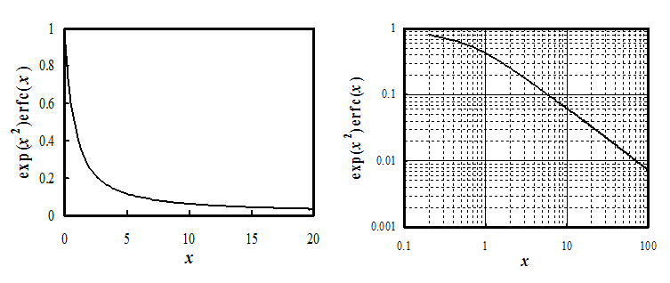
At low values of x the function can be linearized, and current density is given by:
| \( \displaystyle\frac{i(t)}{nF}=k_{ox}c_{\text{R}}^b\left(1-\frac{2\lambda\sqrt{t}}{\sqrt{\pi}}\right) \) | (7.21) |
|---|
Plotting current density as a function of \( \sqrt{t} \) and extrapolating to zero, the intercept at the current axis gives the value of kox. In principle, this could be seen directly from current at t = 0, but this value may be blurred due to the charging current or the limited response time of the potentiostat.
Potential steps are mainly used to determine electrochemical rate constants, as indicated above. In systems in which an electrode reaction is accompanied by a homogeneous reaction, a second step to the reverse potential can be made. The response to the second step now depends on the rate of the homogeneous reactions, which can be utilized in the analysis; these problems are beyond the scope of this book.
7.1.2 Linear potential scan or cyclic voltammetry
Linear potential scan or cyclic voltammetry is probably the most commonly applied electrochemical method. Although its calculus is more complicated than that of a potential step above, and although the accurate determination of kinetic parameters is prone to errors from various sources, it is an excellent semi-quantitative method. With reasonable training and experience, it is easy to deduce what kind of phenomena will prevail in the system. Estimates of the electrode reaction rate and the number of electrons exchanged are readily available, and the presence of an adsorption step or a following homogeneous reaction can easily be detected, for example. More specific reaction mechanisms, such as disproportionation also have their own very characteristic responses. The analysis of an electrochemical system is therefore commonly initiated with potential scans at varying scan rates, after which a more specific method can be chosen that applies to that particular problem.
As the name tells, the
electrode potential is scanned linearly as a function of time. If the scan is
reversed immediately from the end value back to the initial potential, the
procedure is called cyclic voltammetry. The scan rate is usually kept the same
in the forward and backward scans, although this is not mandatory; the theory of
cyclic voltammetry has been developed for constant scan rates. The potential
function in cyclic voltammetry can formally be written as
| \( \displaystyle E=E_i+vt-2H(t-t_s) v(t-t_s) \) | (7.22) |
|---|
where Ei is the initial potential, v the scan rate (\( Vs^{-1} \)), and ts the time of the scan reversal; the corresponding potential is accordingly Es (’s’ = switching). The scan rate v can be either positive or negative. \( H(t-t_s) \) is the Heaviside step function that has the value zero when t < ts and unity when \( t \geq t_s \).
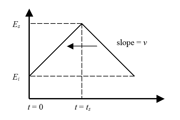
Because the quantity \( \theta \) in Equation (7.5) is no more constant, the
Nernst equation cannot be transformed to the Laplace domain (Equation (7.6)). Instead,
the boundary condition is written as
| \( \displaystyle\frac{c_{\text{O}}(0,t)}{c_{\text{R}}(0,t)}= \theta_ie^{ \sigma t-2H(t-t_s) \sigma(t-t_s)}= \theta_iS(t) \) | (7.23) |
|---|
where \( \theta _i=\text{exp}[\frac{nF}{RT}(E_i-E^{0'})]] \) and \( \sigma=\frac{nF}{RT} v \) ; \( \sigma \) has the dimension s−1. The surface concentrations, Equation (7.4), are transformed back to the time domain using the convolution theorem:
| \( \displaystyle c_{\text{R}}(0,t)=c_{\text{R}}^b-\frac{1}{nF \sqrt{\pi D_{\text{R}}}} \int_{0}^{t}{\frac{i(u)du}{\sqrt{t-u}}} \) | (7.24) |
|---|
| \( \displaystyle c_{\text{O}}(0,t)=c_{\text{O}}^b-\frac{1}{nF \sqrt{\pi D_{\text{O}}}} \int_{0}^{t}{\frac{i(u)du}{\sqrt{t-u}}} \) | (7.25) |
|---|
In the above
equations, u is the dummy time
variable. Inserting Equations (7.24) and (7.25) into Equation (7.23) we find that
| \( \displaystyle\int_{0}^{t}{\frac{i(u)du}{\sqrt{t-u}}}=\frac{nF \sqrt{\pi D_{\text{O}}}}{1+ \xi \theta_iS(t)} \) | (7.26) |
|---|
\( \xi \) is defined earlier. The problem is reduced to the solution of the convolution integral on the left-hand side where the current function resides. In addition, the integral has a singularity at the upper integration limit. Equation (7.26) is written in a dimensionless form for the numeric solution. The time variable u is replaced with a dimensionless potential variable \( \theta= \sigma u \), leading to \( du=d \tau/ \sigma \). The current function i(u) is formally replaced with a new function \( g( \tau) \). The convolution integral is now in the form of
| \( \displaystyle\int_{0}^{t}{\frac{i(u)du}{\sqrt{t-u}}}=\frac{1}{\sqrt{\sigma}} \int_{0}^{\sigma t}{\frac{g(\tau)d \tau}{\sqrt{\sigma t-\tau}}} \) | (7.27) |
|---|
This is further divided by \( nF\sqrt{\pi D_{\text{O}}}c_{\text{O}}^b \), resulting in the dimensionless current function \( \chi( \tau) \):
| \(\displaystyle \int_{0}^{\sigma t}{ \frac{\chi(\tau)d\tau}{\sqrt{\sigma t-\tau}}}=\frac{\theta_iS(t)C_r-1}{1+ \xi \theta_iS(t) }; \chi(\tau)=\frac{g(\tau)}{cFc_{\text{O}}^b \sqrt{\pi D_{\text{O}}\sigma}} \) | (7.28) |
|---|
where \( C_r=c_{\text{O}}^b/c_{\text{R}}^b \). The real physical current (density) is expressed by the dimensionless current (density) as
| \(\displaystyle i(t)=g(\sigma t)=nFc_{\text{O}}^b\sqrt{\pi D_{\text{O}}\sigma}\chi(\sigma t) \) | (7.29) |
|---|
If only species ‘R’ is initially present,\( c_{\text{R}}^b \) is replaced with \( c_{\text{O}}^b \), Cr = 1, and unity vanishes from the numerator of the right hand side of Equation (7.28).
Integral equation (7.28) must be solved numerically. The best known methods is that of Nicholson and Shain in 1964 [1]. Integration by parts removes the singularity at the upper limit:
The
first term on the right-hand side vanishes at the upper limit, and because the
experiments are initiated at the potential where current is zero, it also vanishes at the lower limit. The second term is replaced with a sum, dividing \( \sigma \)t to
subintervals: \( \sigma t=N\delta \) and \( \tau=k\delta \) where
k = 0, 1, 2, ... , N.
Equation (7.31) thus assumes that in the interval [k, k+1] the term \( \sqrt{N-k} \) is nearly constant and can be moved in front of the integral sign, and from here \( d\chi \) can be integrated. Summing is easily done with a computer script. Current is calculated using the values calculated previously:
|
|---|
The numeric solution of the convolution integral gives the following diagnostic criteria for a reversible reaction:
1. The peak current density, ip, is
\( \displaystyle i_p=0.4463nFc_{O}^b\sqrt{\frac{nF}{RT}}\sqrt{v}\sqrt{D_{\text{O}}} \) |
(7.33) |
|---|
Equation (7.33) is known as the Randles-Sevcík equation. It is most often used to determine the diffusion coefficient of a trace ion by plotting peak currents as the function of \( \sqrt{v} \). Alternatively, if the diffusion coefficient is known, the concentration can be calculated.
2. The potential of the peak current, Ep, is related to the half-wave potential, E1/2, with
| \(\displaystyle |E_p-E_{1/2}|=\bigg|E_p-E^{0'}+\frac{RT}{nF}\text{ln} \xi\bigg| =1.109\frac{RT}{nF} \) | (7.34) |
|---|
| \(\displaystyle |E_p-E_{1/2}|=1.09\frac{RT}{nF}=28.0/n \) mV at 25 ºC | (7.35) |
|---|
Ep/2 is the potential at which current is half of the peak current; finding this potential from a graph is easier than Ep because the current peak may be rather flat.
3. The separation between the current peaks in forward and reverse directions, \( \Delta E_p \), is 59/n mV at 25 ºC; this is the diagnostic criterion for the reversibility of an electrochemical reaction.
4. The mid-point of the potentials of the peak currents is ~E1/2.
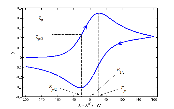
If an electrode reaction has a limited rate, the Nernst equation is replaced by the kinetic equation (6.12) into which the surface concentrations, Equations (7.24) and (7.25) are added. Potential is now included in the rate constants kox and kred, Equation (6.10). The numeric solution is rather cumbersome, so we will only present the results. The sluggishness of an electrode reaction is seen as an increase of \( \Delta E_p \) as the function of the scan rate and as a decrease of the peak currents. Table 7.1 shows n\( \Delta E_p \) as the function of the dimensionless parameter \( \psi \).
| \(\displaystyle \psi=\frac{\xi ^{\alpha /2}k^0}{\sqrt{D_{\text{O}}\pi \sigma}} \) | (7.37) |
|---|
\( \sigma \) and \( k^0 \) are defined in Chapter 6, and \( \xi \) and \( \sigma \) are as above.
As Table 7.1 shows, the peak separation \( \Delta E_p \) is practically the same as in the reversible case when \( \psi \) > 20. A typical value of a diffusion coefficient is of the order of 10-5 cm2 s-1, and since the scan rate cannot be increased without limits – for technical reasons 1 V s−1 often is the upper limit – the upper limit of k0 that can be determined with cyclic voltammetry is of the order of 0.5-1 cm s−1. The accuracy of the analysis based on Table 7.1 is not very good at higher values of \( \psi \): when \( \psi \) decreases from 20 to 5, \( n\Delta E_p \) increases only 4 mV, which is the level of measurement accuracy due to the flatness of the current peaks. Yet cyclic voltammetry is an excellent preliminary method because if we see, for example, that the peak separation increases with the scan rate, we know that the electrode reaction is under kinetic control and we get an estimate for the value of k0. Other techniques such as potential step or impedance spectroscopy can then be used for more accurate determination.
|
Table 7.1. Peak separation as a function of parameter y at 25 ºC23F[2]. |
|
|
y |
n\( \Delta E_p \) (mV) |
|
20 |
61 |
|
7 |
63 |
|
6 |
64 |
|
5 |
65 |
|
4 |
66 |
|
3 |
68 |
|
2 |
72 |
|
1 |
84 |
|
0.75 |
92 |
|
0.50 |
105 |
|
0.35 |
121 |
|
0.25 |
141 |
|
0.10 |
212 |
The left-hand panel of Figure 7.5 shows a few simulated voltammograms with varying values of parameter \( \psi \), keeping the scan limits and a constant. The peak separation \( \Delta E_p \) does not quite correspond to Table 7.1 because the smaller \( \psi \) is, the more sensitive is \( \Delta E_p \) to the switching potential where the scan direction is reversed.
In the right panel, parameter \( \psi \) is kept constant and the value of the charge transfer coefficient a is varied. As can be seen, the effect of \( \alpha \) on the shape of the voltammograms is rather small. Increasing \( \alpha \) increases the oxidation current peak and decreases the reduction current peak. Marcus theory showed that a is not a constant but varies slightly as the function of potential. The value 0.5 is therefore most commonly assumed to be \( \alpha \), which is quite an accurate assumption around the half-wave potential.
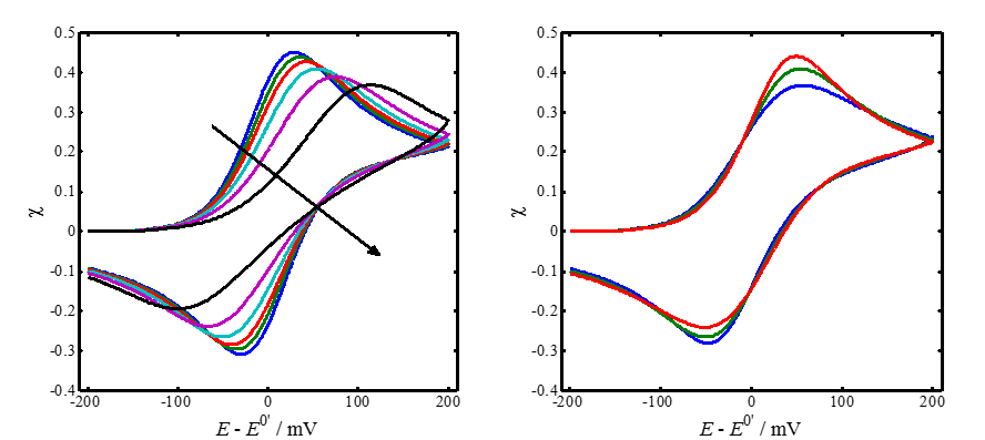 |
|---|
|
Solving more complex reaction mechanisms is easier with
numerical simulations of the transport equations. Let us consider an EC mechanism
where R is first oxidized to O, which then reacts homogeneously further to P:
Let us assume that the electrochemical reaction is reversible and the homogeneous reaction is irreversible, with a rate constant of k. The transport equations are:
The equations above are converted into a dimensionless form with the following change of variables: \( C_i=c_i/c_{\text{R}}^b \), \( z=x/(D\tau) \) and \( T=t/\tau \); \( \tau \) is characteristic time of the measurement, e.g. the duration of the scan, t = 2|Ei – Es|/v. The transport equations now become
The continuity equation on the electrode becomes
The relationship between I(T) and c is easy to calculate when the scan limits, Ei and Es, are known. Equations (7.41) - (7.43) can be solved using various numerical methods.‡ A simulation with varying values of K can be found below
Figure 7.6 shows the characteristics of the EC mechanism:
when the rate of the homogeneous reaction increases or the scan rate decreases, the
reverse current vanishes because the oxidized species ‘O’ formed in the
electrochemical step reacts further to ’P’ to a greater extent, thereby decreasing
the concentration of ‘O’. Hence by measuring the reverse current peak at
varying scan rates, K can be
determined using a simulated working
curve. Such a working curve can represent, for example, the ratio of the
current peaks as a function of K[3].
|
|---|
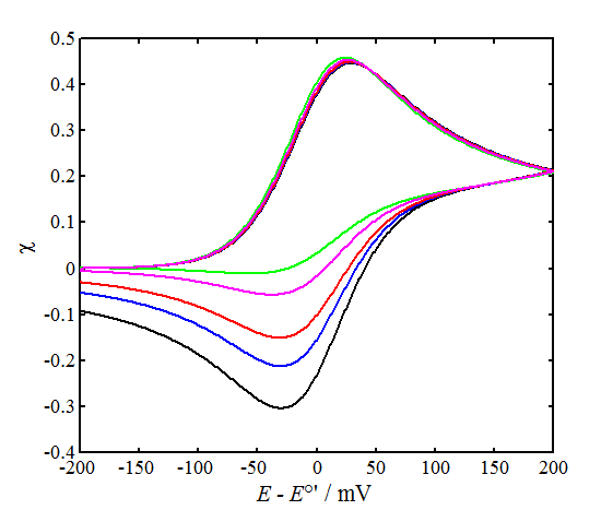
If the peak separation \( \Delta E_p \) is less than 59/n mV, the electrode reaction is probably linked to an adsorption step. If adsorption is the rate-limiting step, the oxidation and reduction current peaks can be found at the same potential and are directly proportional to the scan rate, not to the square root of the scan rate like under diffusion control.
Electrode capacitance Cdl also contributes to the measured current. The capacitive (charging) current, iC, is
| \(\displaystyle i_c=C_{dl}v(1-e^{-t/RC_{dl}}) \) | (7.44) |
|---|
The exponential term of the above equation decays very fast. At solid electrodes, the contribution of the capacitive current is significant only at very high scan rates while at immiscible liquid-liquid interfaces it can be quite high. We derived above that the faradaic current is proportional to the square root of the scan rate. The total current iT is therefore
| \(\displaystyle i_{\text{T}}=A\sqrt{v}+C_{dl}v \Leftrightarrow i_{\text{T}}/\sqrt{v}=A+C_{dl}\sqrt{v} \) |
(7.45) |
|---|
where A is a constant. Plotting \( i_{\text{T}}/\sqrt{v} \) as a function of \( \sqrt{v} \) at each potential, a straight line is obtained with the slope of Cdl. Figure 7.7 shows just such an analysis of the water-1,2-dichloroethane (DCE) interface.
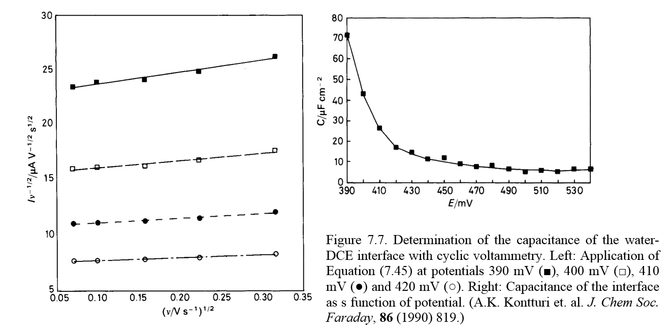
7.1.3. Current step
When constant current is fed to an electrode, the boundary condition of the transport problem is known, making the solution easy. Since the Laplace transform of the constant current density i is i/s, the surface concentrations in the Laplace domain are (only ’R’ initially present)
| \( \displaystyle\bar c_{\text{R}}(0,s)=\frac{c_{\text{R}}^b}{s}-\frac{i}{nF\sqrt{D_{\text{R}}}}\frac{1}{s^{3/2}} \) |
(7.46) |
|---|
| \(\displaystyle \bar c_{\text{O}}(0,s)=\frac{i}{nF\sqrt{D_{\text{O}}}}\frac{1}{s^{3/2}} \) |
(7.47) |
|---|
After inverse transformation,
| \( \displaystyle c_{\text{R}}(0,t)=c_{\text{R}}^b-\frac{2i\sqrt{t}}{nF\sqrt{\pi D_{\text{R}}}} \) | (7.48) |
|---|
| \( \displaystyle c_{\text{O}}(0,t)=\frac{2i\sqrt{t}}{nF\sqrt{\pi D_{\text{O}}}} \) |
(7.49) |
|---|
The moment when the surface concentration of ’R’drops to zero is known as the transition time, \( \tau \). It is given by the Sand equation:
| \( \displaystyle\sqrt{\tau}=\frac{nFc_{\text{R}}^b\sqrt{\pi D_{\text{R}}}}{2i} \) | (7.50) |
|---|
Surface concentrations can be written in a compact form with the transition time:
| \( \displaystyle c_{\text{R}}(0,t)=c_{\text{R}}^b\left(1-\sqrt{t/\tau}\right) \) |
(7.51) |
|---|
| \( \displaystyle c_{\text{R}}(0,t)=c_{\text{R}}^b \xi^{-1}\sqrt{t/\tau} \) | (7.52) |
|---|
|
Calculation of the concentration profiles does not pose a problem either. The profile of ’R’in the Laplace domain is
A comparison of Figures 7.1 and 7.8 reveals the fundamental difference between potential and current steps: potential step fixes the surface concentration and current step the concentration gradient at the surface as a constant. |
|---|
The electrode potential is obtained as a function of time applying Equations (7.51) and (7.52):
| \( \displaystyle E=E^{0'}-\frac{RT}{nF}\text{ln} [ \xi(\sqrt{\frac{\tau}{t}}-1) ] \) | (7.55) |
|---|
Transition time is therefore observed as the point at which the electrode potential changes abruptly. Times t = 0 and \( t=\tau \) are, in principle, singularities of Equation (7.55) but in practice this cannot naturally happen. At these points, something else than the redox couple being investigated defines the electrode potential after transition time, most probably the decomposition of the solvent.
Experimental determination of the transition time is not, however, simple. Since the experiment is not carried out under potential control, the electrode potential may drift before the transition time to the hydrogen (on the cathode) or oxygen evolution region (on the anode). The reduction of metals in particular is only easy on the mercury electrode that has an exceptionally high overpotential of hydrogen evolution.
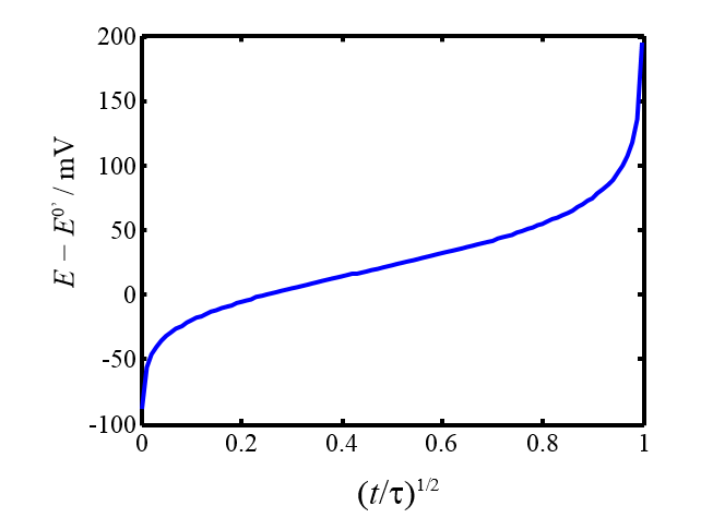
Figure 7.9. Electrode potential as a function of time during a current step experiment; n = 1 and \( \xi \) =1.
Electrode capacitance adds yet another level of difficulty. Capacitive current iC is defined as
| \( \displaystyle i_C=C_{dl}\frac{\partial E}{\partial t} \) | (7.56) |
|---|
Equation (7.56) means that a certain portion of the current is consumed by charging the electric double layer. Since the double layer capacitance Cdl is also a function of the electrode potential, this makes an accurate quantitative analysis of the effect of the capacitance rather difficult.
* The meaning of s is discussed in greater detail in the chapter on the impedance technique; it represents frequency.
† Function y = exp(x2)erfc(x) can be approximated with high accuracy with the polynomial y = 0.34802 z - 0.09587 z2 + 0.74785 z3, where z = (1 + 0.47047 x)-1. From: M. Abramowitz ja I.A. Stegun (Ed.), Handbook of Mathematical Functions, 7. p., Dover, New York, 1970, p. 299.
[1] R.S. Nicholson, I. Shain, Anal. Chem. 36 (1964) 7066.
[2] |Es - Ep| = 112.5/n mV. From: R.S. Nicholson, Anal. Chem. 37 (1965) 1351.
‡ See, e.g. D. Britz, Digital Simulation in Electrochemistry, 2. Ed., Springer, Berlin, 1988.
[3] A.K. Kontturi et al. J Electroanal. Chem. 418 (l996) 131.
7.2. Steady-state methods
In steady-state (or stationary) methods, the concentration does not change as a function of time, i.e. \( \partial c/\partial t =0 \), and Fick’s second law reduces into the form of \( \nabla^2c=0 \). This seems to simplify the solution of the transport problem, but this does not happen in practice because a true steady-state can only be reached without convection in spherical geometry. In this case, the operator \( \nabla^2 \) takes the form
| \( \displaystyle\nabla^2=\frac{\partial^2}{\partial r^2}+\frac{2}{r}\frac{\partial}{\partial r} \) (spherical geometry, no angular dependency) | (7.57) |
|---|
and the concentration profile is
| \( \displaystyle c(r)=A+\frac{B}{r} \) (spherical geometry, no angular dependency) | (7.58) |
|---|
where A and B are constants. In linear geometry, in contrast, the concentration profile would be c(x) = A + Bx, but the boundary condition c(x→ ∞) = cb (or 0) would be absurd because the function A + Bx is not limited. In order to reach a true steady-state, the solution must be stirred resulting in an unstirred stagnant layer is forming on the surface of the electrode due to adhesion between the electrode and solvent molecules; we denote the thickness of this layer as \( \delta \). Now, the boundary condition changed to c(d) = cb (or 0), the transport problem has a meaningful solution in which the concentration changes linearly in the interval [0,\( \delta \)]. The real problem is determining the thickness \( \delta \).
Figure 7.10 shows how the thickness \( \delta \) is usually determined. The rate of the solution flow changes gradually from zero on the surface (non-slip condition) to its maximum value in the bulk. In channel flow, for example, the velocity profile is parabolic. The range of the velocity profile can be an order of magnitude wider than that of the concentration profile. According to Figure 7.10, \( \delta \) is defined as the thickness that is obtained by extrapolating the linear part of the concentration profile to the distance where the concentration would be equal to its bulk value. This is, however, only a thought, a virtual definition, because we cannot measure it. It is therefore evaluated from the solution of the transport problem using the measurable limiting current and assuming that in the region 0 < x < \( \delta \) there is no convection:
| \( \displaystyle c(x)=c^b-\frac{i(\delta-x)}{nFD} \Rightarrow \delta=\frac{nFDc_0}{i_{\text{lim}}} \) | (7.59) |
|---|
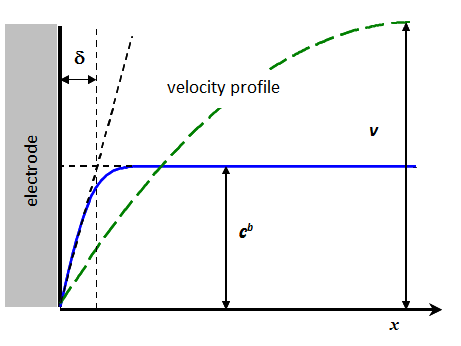
In this way, the Tafel slopes and (apparent) rate constant k0 could be determined, as described in Chapter 6, but in practice, steady-state methods are more sophisticated, taking convection explicitly into account via the solution of the convective diffusion equation
| \( \displaystyle D\nabla^2c-\vec{v}\nabla c=0 \) | (7.60) |
|---|
The solution velocity \( \vec{v} \) must be solved using the Navier-Stokes equation. These methods are therefore also known as hydrodynamic methods. [1] Because of the mathematical complexity of flow dynamics, only rotating disk and channel-flow electrodes are introduced in this book.
7.2.1 Rotating disc electrode (RDE)
When an electrode is rotated a velocity field is formed in its vicinity in a manner illustrated in Figure 7.11. The Navier-Stokes equation has been solved for this case in the form of a power series; we only need the first parabolic term in the series. The velocity profile perpendicular to the electrode surface is
| \( \displaystyle v(x)=-\frac{\omega^3}{v}^{1/2}0.510x^2=-Ax^2 \) | (7.61) |
|---|
where \( \omega \) is the angular frequency of rotation (\( \omega=2\pi f \)) and \( \nu \) is the kinematic viscosity of the solution (\( \eta/\ \rho \), for water ~0.01 cm2/s at 25 °C). At the electrode, the solution is thrown away from the center along the surface, but this velocity component does not contribute to the electric current: current is proportional only to the perpendicular component of the flux. Equation (7.61) also appears to give an absurd result that the velocity v(x) is increasing without limits with increasing distance x. First, the full solution with higher order series terms brings the velocity to zero at long distances and, second, Equation (7.61) applies only in the immediate vicinity of the electrode.
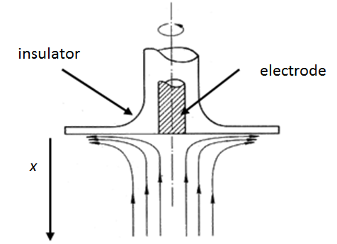
Figure 7.11. Solution flow near a rotating disk electrode.
|
Let us use equation (7.61) as the convection term in the Nernst-Planck equation:
Taking the divergence, the equation of convective diffusion is obtained:
The boundary conditions are c(\( x \rightarrow \infty \)) = cb, v(x=0) = 0, and the usual current boundary condition, Equation (3.48) [2]. Inserting p = dc/dx, the above equation becomes
The integral above can be calculated using the change of variables \( u=\frac{Ax^3}{3D} \Rightarrow dx=(\frac{D}{9A})^{1/3}u^{-2/3}du \). We therefore find the following:
where \( \Gamma \) is the Gamma function or the general factorial function; it is tabulated. It has the property \( \Gamma(m+1)=m\Gamma(m)=m! \). |
|---|
The limiting current density is obtained from Equation (7.66) setting c(x = 0) = 0:
The limiting current density is obtained from Equation (7.66) setting c(x = 0) = 0:
\( \displaystyle i_{\text{lim}}= \mp0.620nFD^{2/3}c^b\omega^{1/2}v^{-1/6} \) |
(7.68) |
|---|
The sign of the current must be chosen according to the reaction, i.e. if it is cathodic (i < 0) or anodic (i > 0). Equation (7.68) is known as the Levich equation and it tells us the important fact that ilim ~\( \omega \)1/2. Since all electrode reactions have a limited rate, an RDE is most suitable for the determination of reaction rate constants.
If current is measured at a potential where i < ilim, Equation (7.66) can be modified in the form of
| \(\displaystyle i=\frac{nFD(c^b-c(x=0))}{\delta} \) |
(7.69) |
|---|
where we have identified the thickness of the diffusion boundary layer \( \delta \) as the group of variables
| \( \displaystyle\delta=1.61D^{1/3}\omega^{-1/2}v^{1/6} \) | (7.70) |
|---|
Analogously to Chapter 6, we can again write the surface concentration as
| \( \displaystyle c(x=0)=c^b(1-i/i_{\text{lim}}) \) | (7.71) |
|---|
Let’s consider an oxidation reaction. Current density is i = nFkox cR(x=0) (only species ‘R’ initially present). Applying Equation (7.71) above, we get the following results:
| \( \displaystyle i=\frac{nFk_{ox}c_{\text{R}}^b}{1+(nFk_{ox}c_{\text{R}}^b)/i_{\text{lim}}} \) \( \displaystyle \frac{1}{i}=\frac{1}{nFk_{ox}c_{\text{R}}^b}+\frac{1}{0.620nFc_{\text{R}}^bD^{2/3}v^{-1/6}\omega^{1/2}}=\frac{1}{i_{\text{kin}}}+\frac{1}{i_{\text{lim}}} \) |
(7.72) |
|---|
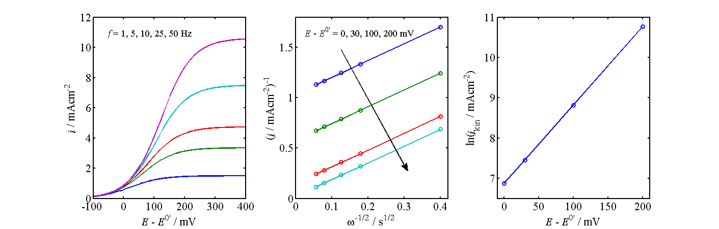
Figure 7.12. Determination of kinetics from the current-voltage curves of an RDE.
The analysis shown in Figure 7.12 proceeds as follows: At selected potentials, the inverse of current (density), i-1, is plotted as a function of \( \omega^{-1/2} \) and this line is extrapolated to zero, in other words to infinite angular frequency; the intercept gives the kinetic current density ikin and thereby kox. Kinetic current is the current that would occur in the absence of mass transfer limitations, ikin = nFkox cRb . A graph representing Equation (7.72) is commonly called as the Koutecký-Levich plot. As shown in the center panel of Figure 7.12, these lines should have the same slope at each potential. Finally, ln(ikin) is plotted as a function of the electrode potential. The slope of this line gives the charge transfer coefficient a, and the intercept at E = E0’ the value of k0.
An RDE has an important modification, a rotating ring-disk electrode (RRDE) in which a concentric ring is placed around the disk at a distance of around 1 mm. Its purpose is to detect species on the ring that are formed on the disk. This can be accomplished, for example, by scanning the disk potential in the cathodic direction and keeping the ring at a constant anodic potential. Any reduced species on the disk are transported immediately to the ring (if they are soluble), where they can be re-oxidized. In this way, reaction mechanisms can be studied when the reaction intermediates are short-lived.
Calculus for the transport problem is rather challenging. An RRDE is calibrated by defining the collector efficiency with a known redox couple, i.e. finding the fraction of the species that is detected on the ring. The collector efficiency depends only on the electrode dimensions and the separation between the disk and the ring. An RRDE requires a bipotentiostat that is capable of controlling the disk and ring potential (or current) separately.
An example of RRDE calibration with a ferro/ferricyanide redox couple is shown below. On the glassy carbon disk, Fe3+ is reduced to Fe2+ whicht is then collected on the platinum ring. The numbers indicate the rotation rate in rpm. The ratio of the ring and disk current, in other words the collector efficiency N ≈ 41%.
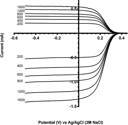
7.2.2 Channel flow electrode
Another hydrodynamic method that has a wide practical use is the channel flow electrode. It is often used as a detector in liquid chromatography, capillary electrophoresis or flow injection analysis. The electrode is placed downstream in the flow channel, after a separation unit, and set at a sufficiently anodic or cathodic potential to oxidize or reduce the analyte on the electrode; it is therefore used under limiting current conditions. A reference electrode is usually placed upstream of the working electrode, while a counter electrode is preferably placed downstream of the working electrode in order to prevent its possible reaction products from being transported to the working electrode.
The transport problem of the channel flow electrode can be solved in a closed form for a rectangular channel because the velocity profile is accurately known. In a fully developed Poiseuille flow, the profile is parabolic with zero velocity on the channel walls that is known as the non-slip condition. The limiting current of a rectangular electrode is given by Equation (7.73), also known as the Levich equation:
| \( \displaystyle I_{lim}=0.925zFD^{2/3}c^bw\left(\frac{l^2\dot{V}}{h^2d}\right)^{1/3} \) | (7.73) |
|---|
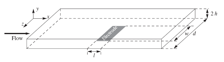
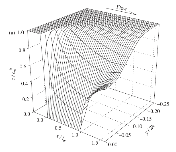
Figure 7.15. Concentration distribution near the channel flow electrode under limiting current conditions. From: Liljeroth et al., J. Electroanal. Chem., 483 (2000) 37.
The coefficient 0.925 in Equation (7.73) is sometimes replaced with 0.835, depending on the simplifying assumptions made in the derivation of the limiting current. The essential feature is, however, that the limiting current is proportional to the cubic root of the volume flow rate. In practice, the electrode response is calibrated using known concentrations, eliminating the significance of the constant coefficients. A detailed description of the solution of the transport problem is available in the literature [3] The problem is to solve first the Navier-Stokes equation and then the convective diffusion Equation (7.60). Figure 7.15 illustrates the concentration distribution of an analyte near the channel flow electrode, solved using the finite element method using Comsol Multiphysics® software. Although all transport problems can today be solved numerically without simplifying assumptions and in an arbitrary geometry, a closed form solution has the advantage that it provides the dependence of, say, the limiting current on the relevant variables explicitly.
[1] A classical textbook of hydrodynamic methods is: V.G. Levich, Physicochemical Hydrodynamics, Prentice Hall, Englewood Cliffs NJ, 1962.
[2] Think: why we are allowed to take the upper boundary condition at x → ∞, instead of x = d?
[3] K. Kontturi, L. Murtomäki, J.A. Manzanares, Ionic Transport Processes, Oxford University Press, 2009.
7.3. Ultramicroelectrodes
If a dimension of an electrode is of the order of microns or less, the electrode is called an ultramicroelectrode. The purpose of an ultramicroelectrode is firstly to enhance the rate of mass transfer, which makes the determination of fast reaction kinetics feasible, and secondly to reduce the electric current, which makes ohmic losses insignificant in non-aqueous solutions too.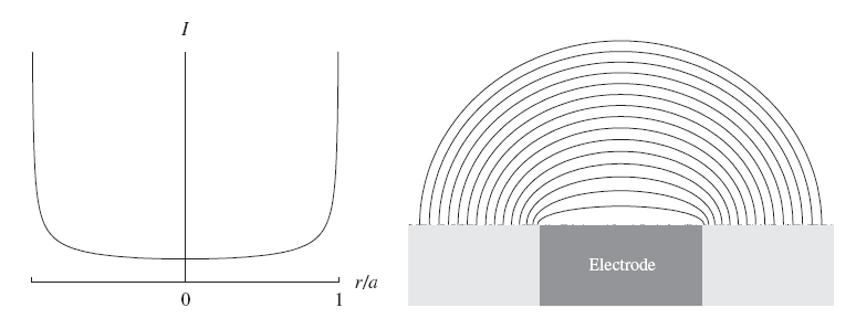
Figure 7.16. Radial current distribution (left) and equi-concentration lines (right) on a disk electrode.
As can be seen in Figure 7.16, the local current density increases very significantly towards the electrode edges. It can be shown that the radial distribution under mass transfer control is of the form
| \( \displaystyle i\propto\frac{1}{\sqrt{1-(r/a)^2}} \) | (7.74) |
|---|
where a is the disk radius. The current density is therefore in principle, unlimited at the edge r = a, but the integral over the disk remains limited. In reality, current density is kinetically limited at the edge of the disk. When the disk radius a is reduced down to a few microns, the concentration profile becomes nearly spherically symmetrical (see the right-hand panel of Figure 7.16), and Equation (7.57) can be used.
Ultramicroelectrodes are used in both transient and steady-state methods. In a steady-state, Equation (7.58) gives with the boundary conditions c(\( r \rightarrow \infty \)) = cb and c(r = a) = 0 the concentration profile
| \( \displaystyle c(r)=c^b(1-a/r) \) | (7.75) |
|---|
and the limiting current density
| \(\displaystyle i_{\text{lim}}=\pm nFD\left(\frac{dc}{dr}\right)_{r=a}=\pm nFD(c^b/a) \) | (7.76) |
|---|
If the electrode really were a hemisphere, the limiting current would be \( I_{\text{lim}}=\pm2\pi nFDc^ba \), but Fleischmann and Pons have shown [1] that the limiting current of a disk ultramicroelectrode is
| \( \displaystyle I_{\text{lim}}=\pm4nFDc^ba \) | (7.77) |
|---|
In practice, calculations are made in spherical geometry and the results are corrected as above.
In transient methods, the general Equation (7.4) takes the form
| \( \displaystyle\bar c_i(0,s)=\frac{c_i^b}{s}+ \frac{\bar i (s)}{nF\sqrt{D_i}(\sqrt{s}+\sqrt{D_i}/a)} \) | (7.78) |
|---|
proving that when \( a \rightarrow \infty \) the problem returns to linear geometry. Setting the surface concentration to zero, current density in a potential step experiment is in the Laplace domain
| \( \displaystyle\vec{i}(s)=\pm nF\sqrt{D}c^b\left(\frac{1}{\sqrt{s}}+\frac{1}{s}\frac{\sqrt{D}}{a}\right) \) | (7.79) |
|---|
After inverse transformation the result is
| \(\displaystyle i(t)=\pm nF\sqrt{D}c^b\left(\frac{1}{\sqrt{\pi t}}+\frac{\sqrt{D}}{a}\right) \) |
(7.80) |
|---|
Comparing this result with the Cottrell equation (7.11) of linear geometry, it is seen that the current density levels out after the transient period to Equation (7.76), contrary to the Cottrell equation in which the current decays to zero.
Figure 7.17. Current transients (7.76). For the Cottrell equation (7.11), \( \sqrt{D}/a=0 \).
Cyclic voltammograms of an ultramicroelectrode have an interesting feature that if the scan rate is low enough compared to the parameter D/a2, current is practically equal to that in a steady-state, like in Figure 6.3. When the scan rate is increased, the typical shape of a cyclic voltammogram, Figure 7.4, begins to emerge.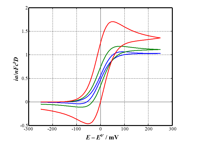
Figure 7.18. Cyclic voltammograms of an ultramicroelectrode at varying scan rates: v = 0.01 (blue), 0.1 (green) and 1.0 (red) Vs-1; electrode radius a = 10 \( \mu \)m.
[1] M. Fleischmann, S. Pons, in: D.R. Rolison, P.P. Schmidt (Eds.), Ultramicroelectrodes, Datatech Systems, Morganton, N.C., 1987.
8. Impedance technique
Impedance technique or impedance spectroscopy is one of the essential methods in modern electrochemistry. It is conceptually very different from other electrochemical techniques and thus deserves its own chapter. In the impedance technique, only a very small periodic perturbation is applied either at equilibrium or in a steady-state, and the output signal caused by the input signal is measured as a function of frequency. A sinusoidal signal is generally used as an input, but in principle, you could also choose a triangular or square waveform input instead. A typical experimental arrangement of an impedance measurement is shown schematically in Figure 8.1.
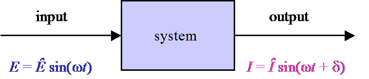
Figure 8.1. Principle of an impedance measurement.
When a voltage signal operating with angular frequency \( \omega \) and amplitude \( \hat{E} \) is applied, a current with an amplitude \( \hat{I} \) is produced in the system. The angular frequency of the signal remains constant while there is a phase shift \( \delta \) between the input and output signals. All the information about the system is included in the phase shift \( \delta \) and the ratio of the amplitudes \( \hat{Z}=\hat{E}/\hat{I} \) as a function of angular frequency.
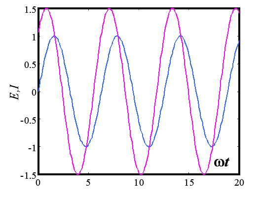
Presenting
data as a function of time as in Figure 8.2 is rather impractical and
pointless, since periodical signals repeat themselves and all the information
can be extracted from a single period (cycle). A sinusoidal signal
is therefore traditionally presented in terms of complex notation. Instead of the
notation in Figure 8.2, voltage and current can be expressed in polar
coordinates as
| \( \displaystyle E=\hat{E}e^{j\omega t} \) | |
| \(\displaystyle I=\hat{I}e^{j(\omega t+\delta)}
\) |
(8.1) |
|---|
where j is imaginary, that is \( j=\sqrt{-1} \) [1]. Graphical representation of the complex notation is shown in Figure 8.3. The fundamental message of expressions (8.1) and Figure 8.3 is that the periodic signal does not change its value as a function of time, but is constant (\( \hat{E} \) or \( \hat{I} \)). However, its phase angle with respect to real axis, i.e. the projection to the real world, changes periodically as the vector rotates about the origin with an angular frequency \( \omega \).
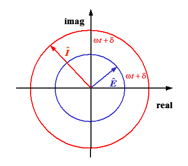
The real and imaginary parts of the complex number z can be obtained from Euler’s formula:[2]
| \( \displaystyle z=\hat{z}e^{\pm j\varphi}=\hat{z}(\cos\varphi\pm j\sin\varphi) \) | (8.2) |
|---|
thus the sinusoidal signal is no more than the real part of a signal in the complex notation. Using Ohm’s law
| \( \displaystyle Z= \frac{E}{I} \) | (8.3) |
|---|
the complex impedance vector can be found to be
| \(\displaystyle Z=\frac{\hat{E}e^{j\omega t}}{\hat{I}e^{j(\omega t+\delta)}}=\frac{\hat{E}}{\hat{I}}e^{-j\delta}=\hat{Z}e^{-j\delta} \) | (8.4) |
|---|
The reciprocal of impedance Y = Z-1 is called admittance, and sometimes both of them combined are called immittance.
The message of equation (8.4) is very significant and profound: the time variable t has disappeared. The amplitude \( \hat{Z} \) and phase shift \( \delta \) depend only on the angular frequency \( \omega \), and thus the impedance of an electrochemical system must be calculated in the frequency domain instead of the time domain used in all other electrochemical methods. The time-dependent signal can be converted to the frequency domain using Laplace transform methods because the Laplace variable s is actually a complex number \( s=\sigma+j\omega \), but we have (arbitrarily) chosen \( \sigma=0 \).
|
In control systems engineering, all analyses are done in the Laplace domain. Let us denote the input in Figure 9.1 as U(s) and output as O(s). The relation between them is written as
where H(s) is the transfer function of a system, which tells us how the input signal is converted to the output signal by the system. The transfer function is a characteristic feature of a system, and thus U(s) can be arbitrary. The characteristics of a transfer function can be studied in the frequency domain by interpreting \( s=j\omega \). We therefore conclude analogously that the admittance Y of an electrochemical system is equal to its transfer function because according to Ohm’s law
If we choose a unit impulse as an input function, the output is equal to the transfer function because the Laplace transform of a unit impulse is U(s) = 1. |
|---|
Later in this chapter, we will present a method based on Laplace transformation that allows us to simplify the impedance analysis largely so that we do not have to write any of the periodic functions or any other forms of functions explicitly. However, some basic elements are easier to introduce using the complex notation as shown in the next subchapter.
[1] The symbol i usually stands for the imaginary unit, but now it is reserved for current density.
[2] More relations of complex numbers can be found
in 13.3. Relations of complex numbers.
8.1. Basic elements of impedance
A resistor R (electric resistance) is always present in an electrochemical system. Ohm’s law states that if the voltage across a resistor is E, the current through the resistor is E/R. The impedance of the resistor is therefore R.
An electrochemical reaction always takes place at the phase boundary, i.e. on the surface of an electrode or catalytic particle in a membrane. At the phase boundary, the electroneutrality condition is not complied with, but the phase boundary has an ability to store electric charge, i.e. it acts as a capacitor. The voltage across a phase boundary gives rise not only to charge transfer, i.e. current I = E/R, but also to the reorganization of charges at the phase boundary. This capacitive current can be expressed as
| \( \displaystyle I_C=C_{dl}\frac{dE}{dt}=j\omega C_{dl}E \) | (8.6) |
|---|
Capacitive impedance is obtained using simple algebra:
| \( \displaystyle Z_C=\frac{1}{j\omega C} \) | (8.7) |
|---|
Since total current across the phase boundary, IT, is IT = E/R + jwCE = (1/R + jwC)E, the admittance of the phase boundary is Y = 1/R + jwCdl and the impedance Z = Y-1. Parallel combination of the charge transfer resistance Rct and double layer capacitance Cdl is therefore the simplest model of an electrode or some other phase boundary as shown in Figure 8.4.
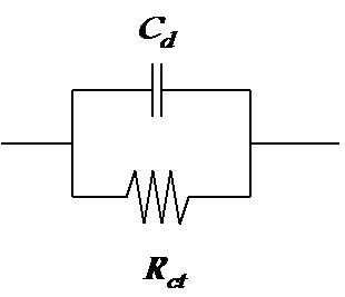
Models of phenomena in dissolving processes, i.e. corrosion, may include also inductors. In this case, the relationship between voltage and current is expressed as:
| \( \displaystyle i=\frac{1}{L} \int Edt=\frac{1}{j\omega L} E \Rightarrow Z_L =j\omega L \) | (8.8) |
|---|
This gives us useful hints on how to determine the total impedance of a multicomponent system. The rule is to sum up the impedances of the components in series and the admittances of the components in parallel as shown in Figure 8.5.
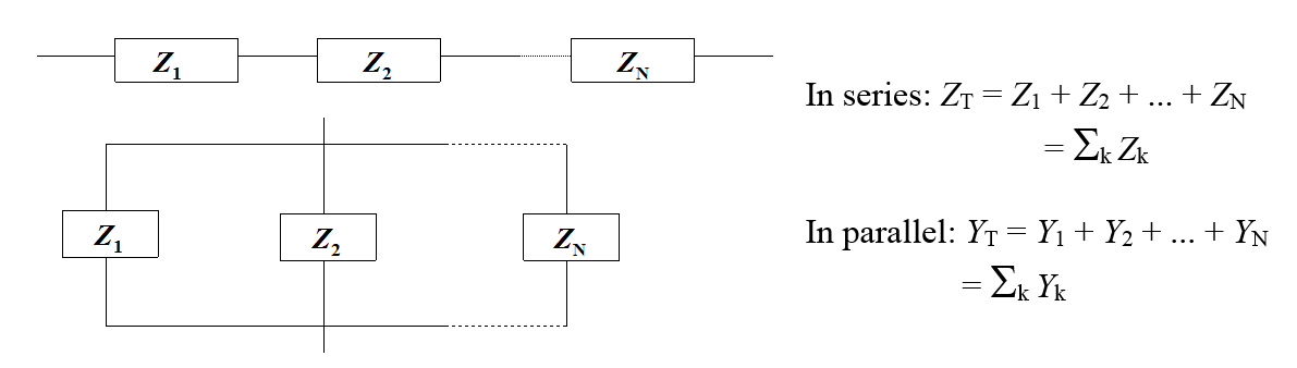
Figure 8.5. Calculation of a total impedance from component impedances.
As the impedance of a resistor is real and that of a capacitor is imaginary, any given impedance can be expressed in terms of a resistor and capacitor in parallel:
| \( \displaystyle Z=R_p+1/j\omega C_p=R_p-j/\omega C_p \) | (8.9) |
|---|
In Equation (8.9), Rp and Cp
are so-called pseudo resistance and capacitance. They are of course functions
of frequency, which explains the use of the prefix ’pseudo’. Sometimes the
imaginary part of an impedance is called reactance. The classical impedance
measurement technique is based on an application of Equation (8.9). In this
method, a very precise impedance bridge is used as shown in Figure 9.6.
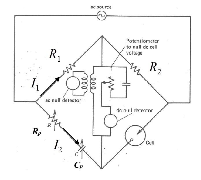
In the middle of the bridge, there are null detectors for both DC and AC. The idea of the measurement is to adjust the values of Rp and Cp so no current is detected at the null detectors between the upper and lower arm of the bridge. When the bridge is at equilibrium, the upper and lower arms are at the same potential and Kirchoff’s second rule can be used to write the equilibrium condition as
\( \begin{cases}I_1R_1=I_2(R_p-j/\omega C_p)\\I_1R_2=I_2Z\end{cases} \)
where R1
and R2 are known resistors
and Z the impedance of the cell studied. Dividing both sides of the equations, impedance Z is obtained:
| \( \displaystyle\frac{R_1}{R_2}=\frac{R_p-j/\omega C_p}{Z} \) | (8.10) |
|---|
Setting R1 = R2 results in Equation (8.9).
The series combination of an inductor and the capacitance brings about an interesting effect: resonance. The total impedance is a sum
| \( \displaystyle Z=j\omega L+(j\omega C)^{-1}=j(\omega L-1/\omega C)=j\frac{\omega^2LC-1}{\omega C} \) | (8.11) |
|---|
Thus, if frequency \( \omega=(LC)^{-1/2} \), impedance is explicitly lost, i.e. the circuit is in resonance. This phenomenon is used for example in radio detectors or quartz crystal microbalances. The circuit includes also a resistor to restrict the current.
|
The basis
of a quartz crystal microbalance relies on the resonance phenomenon. A voltage
of a couple of volts is set across a thin quartz crystal, whereupon the crystal
starts to vibrate due to the piezoelectric effect, i.e. the planes in the
crystal structure start to move with respect to one another. Typical crystals
used in microbalances oscillate at 5 or 10 MHz resonant frequency. When a small
mass is deposited on the crystal, the oscillation frequency becomes smaller
according to Sauerbrey equation:
where \( \Delta f \) is the change in frequency (Hz), f0 is the resonant frequency of a clean crystal, N = 166.8 kHz cm, \( \rho_q \) density of quartz, 2.648 g cm-3, ja \( \Delta m \) mass deposited on the crystal. E.g. Adding a mass of 10 ng cm-2 to a 10 MHz crystal, for example, changes frequency 2.26 Hz. The most sensitive microbalances can easily resolve an added mass of 1 ng cm-2. Both changes in mass and the viscoelastic
properties of a film can be measured using QCM. The analysis is based on the
admittance analysis using a Butterworth-van Dyke circuit, which describes the
oscillation of the crystal.
In the circuit, C0
is the capacitance of the crystal and the lower arm describes the
resonant phenomenon; the admittance of the lower arm has a sharp peak at the
resonance frequency. The values of R, L, and C can be related to the density
and viscosity of the layer based on a very complex theory [1].
The layer must be at
least 100 \( \mu \)m in thickness for the viscoelastic behavior to be able to be observed. If the crystal is in solution, the density
and viscosity of the solution have a similar effect on the crystal as a viscous
layer on the surface. The change in admittance when the crystal is submerged in
aqueous solutions of glycerol with varying concentrations is shown in Figure 9.8.
Figure 8.8. Admittance and phase angle of a quartz crystal as a function of environment,
and density-viscosity product of contacting fluid \( \rho\eta \) (g2 cm-4 s-1). A: air, \( \rho\eta \) = 2\( \times \)10-7; B: water, \( \rho\eta \) = 0.010; C:
43 % glycerol, \( \rho\eta \) =
0.044; D: 64 % glycerol, \( \rho\eta \) = 0,15; E: 80
% glycerol, \( \rho\eta \) =
0.72. Source: see footnote. The dissipation factor D, or ratio of dissipation energy Ediss of the mechanical energy stored in the film, Estored is easy to determine using the values of circuit components in the model:
The quartz crystal is frequently coated with gold to allow for its use as an electrode. Combining mass data with electrochemical data makes it possible to distinguish between the responses of an electroactive and neutral species, which is important in research of conducting polymers. The method is called an electrochemical quartz crystal microbalance (EQCM). |
|---|
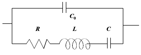
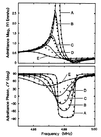
[1] S.J. Martin, V.E. Granstaff, G.C. Frye, “Characterization of a Quartz Crystal Microbalance with Simultaneous Mass and Liquid Loading”, Anal.Chem. 63 (1991) 2272.
8.2. Graphical representations of impedance
Impedance is a complex quantity, so one numerical value is not enough to describe it. There are many ways to represent impedance data [1], but the most common ones are Bode and Nyquist plots. A Bode plot, which is most commonly used in control systems and electrical engineering, shows the magnitude of impedance and the phase angle as a function of logarithm of frequency. The magnitude is commonly expressed in decibels, i.e. 20\( \times \)log|Z|. The phase angle has little relevance in control systems and electrical engineering.
Electrochemists prefer the a Nyquist plot
or impedance plot, in which the real part of impedance Z’ is on the horizontal axis and the opposite number of the
imaginary part -Z” is on the vertical axis at
each frequency. This is because the imaginary part is usually negative.
Frequency is not displayed explicitly in the Nyquist plot.
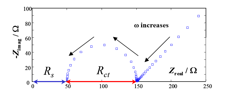
Figure 8.9. Nyquist (impedance) plot of Randles circuit.
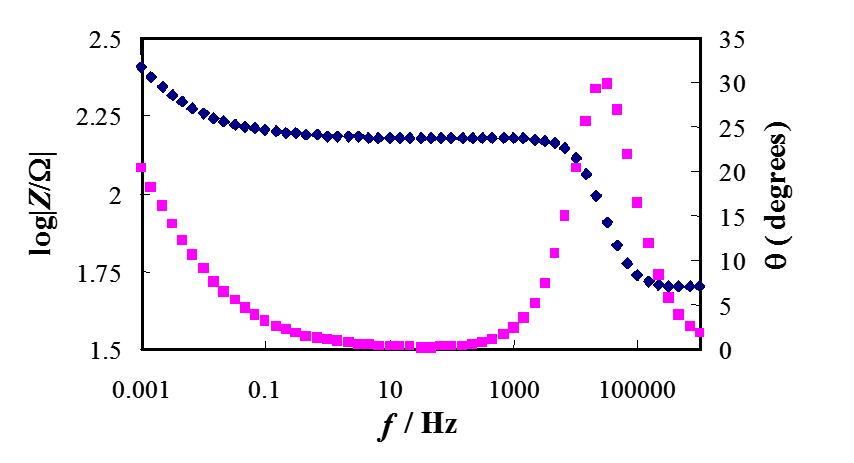
Figure 8.10. Bode plot of Randles circuit. Blue is the magnitude and pink is the phase angle.
The Nyquist and Bode plots of Randles circuit, one of the essential equivalent circuits describing electrochemical systems, is shown in Figures 8.9 and 8.10. For the authors of this book at least, the former is more informative because the ohmic resistance and charge transfer resistance, in other words the rate of charge transfer process, can be seen immediately. Bode plots are monotonically decreasing curves, in which the information is hidden in the negative slope and the points of inflection where the slope changes. In control systems engineering, the so called poles are of great interest, and this information can be obtained from the point of inflection. In this book, we will use almost exclusively Nyquist plots because of their clarity. Sometimes, however, it is more beneficial to show an admittance plot where the real part of admittance is on the horizontal axis and the imaginary part on the vertical axis.
[1] See for example impedance analysis program ‘Equivalent Circuit’ by Bernard A. Boukamp, which has been integrated as a part of the control and analysis program Autolab.
8.3. Determining the impedance of an electrochemical system
We have previously stated that impedance is a frequency-dependent quantity and therefore the most convenient and reasonable way to determine it is in the frequency domain. The conversion from a time variable to a frequency variable is done using Laplace transformation, and because of this, we start with a couple of important remarks concerning Laplace transforms [1]. The Laplace transform is a linear operator:
| \( \mathcal{L}\{af(t)+bg(t)\}=a\mathcal{L}\{f(t)\}+b\mathcal{L}\{g(t)\}=a\overline{F}(s)+b\overline{G}(s) \) |
|
| \( \mathcal{L}\{f(t)g(t)\} \neq \mathcal{L}\{f(t)\}\mathcal{L}\{g(t)\} \) |
(8.14) |
|---|
The symbol \( \mathcal{L} \) represents the Laplace transform, a and b are constants, and f(t) and g(t) arbitrary functions of time; \( \overline{F}(s) \) and \( \overline{G}(s) \) are transforms of f(t) and g(t). The bar over the function highlights the frequency domain and s is the Laplace variable (frequency).
The
transform being linear means that non-linear factors, such as product kf cs cannot be
converted (kf is a
potential dependent rate constant and cs
surface concentration of the reacting species). Non-linear factors therefore have to
be linearized near measurement potential, and because of this, the magnitude of
the input signal has to be small enough for a valid linearization. A few
examples of the most common linearizations are shown in the following
subchapters. Impedance of any given system can be determined following the
steps below:
|
1. Linearize the current-voltage equation. 2. Solve the problem in Laplace domain. 3. Remove non-periodical components of the solution with the relation
4. Impedance is \(\displaystyle Z=\frac{E(j\omega)}{I(j\omega)} \) |
|---|
The third step deserves a couple of remarks. The Laplace transform of a sinusoidal signal takes the form \( 1/(s^2+\omega^2) \), so multiplication with a binomial \( (s^2+\omega^2) \) removes the denominator. All other signals without such a denominator approach zero at the limit \( s=j\omega \). Actually, there is no need to apply Equation (8.15) in practice because all terms without \( \overline{E}(s) \)or \( \overline{I}(s) \) can be eliminated. The following examples will clarify the method.
8.3.1 Linearization of current-voltage curves and faradaic impedance
Current-overpotential equation (6.27) was derived in Chapter 6:
| \( \displaystyle\frac{i}{i_0}=\frac{c_{\text{R}}^s}{c_{\text{R,0}}^b}e^{\alpha nf\eta}-\frac{c_{\text{O}}^s}{c_{\text{O,0}}^b}e^{(\alpha-1) nf\eta} \) | (6.27) |
|---|
Let us linearize this equation at the point of equilibrium \( (i=0, \eta=0, c_{\text{R}}^s=c_{\text{R,0}}, c_{\text{O}}^s=c_{\text{O,0}}) \):
| \( \displaystyle\left(\frac{\partial(i/i_0)}{\partial c_{\text{R}}^s}\right)_{eq}=\frac{1}{c_{\text{R}}^b} ;\left(\frac{\partial(i/i_0)}{\partial c_{\text{O}}^s}\right)_{eq}=-\frac{1}{c_{\text{O}}^b} \) | (8.16) |
|---|
| \( \displaystyle\left(\frac{\partial(i/i_0)}{\partial\eta}\right)_{eq}=\alpha f-(\alpha-1)f=f \) |
|
| \( \displaystyle\frac{i}{i_0} \approx\frac{c_{\text{R}}^s-c_{\text{R,0}}}{c_{\text{R,0}}} -\frac{c_{\text{O}}^s-c_{\text{O,0}}}{c_{\text{O,0}}}+f\eta=\frac{c_{\text{R}}^s}{c_{\text{R,0}}}-\frac{c_{\text{O}}^s}{c_{\text{O,0}}}+f\eta \) |
(8.17) |
|---|
Equation (8.17) can be written directly in the
Laplace domain as follows:
| \( \displaystyle\overline{\eta}(s)=\frac{RT}{nF}\left(\frac{\overline{i}(s)}{i_0}-\frac{\overline{c}_{\text{R}}^s(s)}{c_{\text{R,0}}}+\frac{\overline{c}_{\text{O}}^s(s)}{c_{\text{O,0}}}\right) \) | (8.18) |
|---|
Now we need to determine the surface
concentrations \( \overline{c}_{\text{R}}^s(s) \) and \( \overline{c}_{\text{O}}^s(s) \) from the
transfer equations, which we already did in Chapter 7. Substituting
Equations (7.7) and (7.8) to Equation (8.18) gives
| \( \displaystyle\overline{\eta}(s)=\frac{RT}{nF}\left(\frac{\overline{i}(s)}{i_0}+\frac{\overline{i}(s)}{nFc_{\text{R,0}}\sqrt{sD_{\text{R}}}}+\frac{\overline{i}(s)}{nFc_{\text{R,0}}\sqrt{sD_{\text{O}}}}\right) \) | (8.19) |
|---|
Dividing Equation (8.19) by \( \overline{i}(s) \) and replacing s with \( j\omega \), impedance can easily be found:
| \( \displaystyle Z=\frac{RT}{nFAi_0}+\frac{RT}{n^2F^2A}\left(\frac{1}{c_{\text{R,0}}\sqrt{D_{\text{R}}}}+\frac{1}{c_{\text{O,0}}\sqrt{D_{\text{O}}}}\right)\frac{1}{\sqrt{j\omega}} \) | (8.20) |
|---|
Note that because i stands for current density, we needed to divide the expression by
the area A. The first term of
Equation (8.20) represents charge transfer resistance, Rct. The rate constant of the reaction, k0, can be
determined by substituting the expression for the exchange current density in
Equation (8.20). The latter term of the equation is known as the Warburg element,
which describes diffusion. Because \( j^{1/2}=(1-j)/\sqrt{2} \), it is evident
that the real and imaginary parts of the Warburg element are equal. The
faradaic impedance of the electrode reaction, Zf, is therefore
| \( \displaystyle Z_f=R_{ct}+\frac{\sigma}{\sqrt{\omega}}(1-j) \) | (8.21) |
|---|
where \( \sigma \) is the Warburg element
| \( \displaystyle\sigma=\frac{RT}{n^2F^2A\sqrt{2}}\left(\frac{1}{c_{\text{R,0}}\sqrt{D_{\text{R}}}}+\frac{1}{c_{\text{O,0}}\sqrt{D_{\text{O}}}}\right) \) |
(8.22) |
|---|
The characteristic feature of Warburg
impedance is an increasing straight line at an angle of 45 degrees. When
faradaic impedance and electrode capacitance are in parallel and the solution
resistance is added in front of the whole circuit, an impedance plot shown in
Figure 8.9 is obtained. The whole circuit is called the Randles circuit or Randles
equivalent circuit, shown in Figure 8.11.
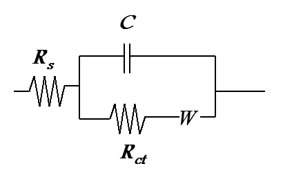
Figure 8.9 shows how the values for Rs and Rct can easily be obtained. The semicircle and the straight line are usually overlapping, so only the left-hand side (high frequencies) of the semicircle is visible. Despite this, it is easy to determine the numerical values using modern software; we will come back to the fitting of circuit components later in this Chapter.
If the solution resistance and capacitance have been eliminated from the experimental data, the residual faradaic impedance can be divided into real and imaginary parts:
| \( \displaystyle Z_f'=R_{ct}+\sigma/\sqrt{\omega} \) |
|
| \( \displaystyle Z_f''=\sigma/\sqrt{\omega} \) |
(8.23) |
|---|
Plotting the real and imaginary parts as a function of \( 1/\sqrt{\omega} \), two straight lines are obtained. Of these two, the real part intersects the vertical axis at Rct and the imaginary part at the origin. Both of the lines have a gradient of s. The plot is sometimes called the Randles plot.
If the impedance measurement is conducted off the equilibrium point, the measurement arrangement has to be such that a real stationary state can be reached (see comments at the beginning of Chapter 7.2). If the experiment is fast enough (< 1 min), we can compromise this requirement because the conditions during the experiment are nearly constant. Linearization is easier straight from the Butler-Volmer equation
| \( \displaystyle\frac{i}{nF}=k_{f}c_{\text{R}}^s-k_{b}c_{\text{O}}^s \) | (8.24) |
|---|
which will, after linearization and using the Laplace transform, take the form
| \( \displaystyle\frac{\Delta\overline{i}(s)}{nF}=k_{f}\Delta\overline c_{\text{R}}^s(s)-k_{b}\Delta\overline c_{\text{O}}^s(s)+\left((1-\alpha)k_{f}c_{\text{R}}^s+\alpha k_{b}c_{\text{R}}^s\right)f\Delta\overline{E}(s) \) | (8.25) |
|---|
Quantities \( \Delta\overline{c}_{\text{R,O}}^s(s) \) represent the deviation from the surface concentration caused by the AC input and are determined by the constant current at each data point, see Equation (7.55); \( \Delta\overline{i}(s) \) and \( \Delta\overline{E}(s) \) are the deviations from constant current and voltage, i.e. amplitudes of the AC signal.
Deviations from the surface concentrations are obtained as usual:
| \( \displaystyle\Delta\overline{c}_{\text{R}}^s(s)=-\frac{\Delta\overline{i}(s)}{nF\sqrt{sD_{\text{R}}}} \) ; \( \Delta\overline{c}_{\text{O}}^s(s)=\frac{\Delta\overline{i}(s)}{nF\sqrt{sD_{\text{O}}}} \) |
(8.26) |
|---|
We substitute Equation (8.26) in Equation (8.25) and place the current and voltage terms on different sides of the equation:
| \( \displaystyle\Delta\overline{I}(s)\left(1+\frac{k_{f}}{\sqrt{sD_{\text{R}}}}+\frac{k_{b}}{\sqrt{sD_{\text{O}}}}\right)=\left((1-\alpha)k_{f}c_{\text{R}}^s+\alpha k_{b}c_{\text{R}}^s\right)\frac{n^2F^2A}{RT}\Delta\overline{E}(s) \) | (8.27) |
|---|
After little rearrangement, impedance is expressed as
| \( \displaystyle Z=\frac{RT}{n^2F^2A} \cdot\frac{1+\lambda/\sqrt{j\omega}}{(1-\alpha)k_fc_{\text{R}}^s+\alpha k_bc_{\text{O}}^s}=R_{ct}\left(1+\frac{\lambda}{\sqrt{j\omega}}\right) \) | (8.28) |
|---|
where parameter \( \displaystyle\lambda=\frac{k_f}{\sqrt{D_{\text{R}}}}+\frac{k_b}{\sqrt{D_{\text{O}}}} \).
Surface concentrations of the stationary state \( c_{\text{R}}^s \) and \( c_{\text{O}}^s \) can naturally be determined from Equation (6.18), but if we want to see how the charge transfer resistance and Warburg element change as a function of potential, we will first sum up the surface concentrations using the general equations (7.7) and (7.8):
| \( \displaystyle\sqrt{D_{\text{R}}}\overline{c}_{\text{R}}^s(s)+\sqrt{D_{\text{O}}}\overline{c}_{\text{O}}^s(s)=\sqrt{D_{\text{R}}}\frac{c_{\text{R,0}}}{s}+\sqrt{D_{\text{O}}}\frac{c_{\text{O,0}}}{s} \Rightarrow \sqrt{D_{\text{R}}}c_{\text{R}}^s+\sqrt{D_{\text{O}}}c_{\text{O}}^s=\sqrt{D_{\text{R}}}c_{\text{R,0}}+\sqrt{D_{\text{O}}}c_{\text{O,0}} \Rightarrow c_{\text{R}}^s=c_{\text{R,0}}+ \xi(c_{\text{O,0}}- c_{\text{O}}^s) \) ; \( \xi=\sqrt{D_{\text{O}}/D_{\text{R}}} \) |
(8.29) |
|---|
The surface concentrations can be determined using Equation (8.24), taking into account that \( k_f=k^0\theta^{1-\alpha} \) and \( k_b=k^0\theta^{-\alpha} \); \( \theta \) is defined in Equation (7.5).
| \( \displaystyle c_{\text{R}}^s=\frac{c_{\text{R,0}}+\xi c_{\text{O,0}}+\xi\theta^\alpha i/Fk^0}{1+\xi\theta} \approx\frac{c_{\text{R,0}}+\xi c_{\text{O,0}}}{1+\xi\theta} \) |
(8.30) |
| \( \displaystyle c_{\text{O}}^s=\frac{\theta(c_{\text{R,0}}+\xi c_{\text{O,0}})-\theta^\alpha i/Fk^0}{1+\xi\theta} \approx\frac{\theta(c_{\text{R,0}}+\xi c_{\text{O,0}})}{1+\xi\theta} \) |
(8.31) |
|---|
Approximation, which eliminates the final term of the numerator, is based on practical experience: There is no point in running impedance measurements with high DC current densities because of the formation of convective currents. The term i/Fk0 is no more than 10-5 mol cm-3 in magnitude. It is possible to derive the results (8.30) and (8.31) directly from the assumption that the surface concentrations follow the Nernst equation; in fact, this assumption is typically made in AC voltammetry.
We can now write the charge transfer resistance and the potential dependency of Warburg element explicitly:
| \( \displaystyle R_{ct}=\frac{RT}{n^2F^2Ak^0(c_{\text{R,0}}+\xi c_{\text{O,0}})} \cdot\frac{1+\xi\theta}{\theta^{1-\alpha}} \) |
(8.32) |
| \( \displaystyle W=\frac{RT}{n^2F^2A(c_{\text{R,0}}+\xi c_{\text{O,0}})\sqrt{D_\text{O}\sqrt{2\omega}}} \cdot\frac{(1+\xi\theta)^2}{\theta}(1-j) \) | (8.33) |
|---|
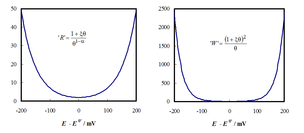
Figure 8.12. Potential dependency of charge transfer resistance (left) and Warburg element (right) without their constants. \( \xi \) = 1 and n = 1; \( \theta \) = exp[(nF)/(RT)(E - E0’)].
The value of the Warburg element becomes two orders of magnitude greater than that of the charge transfer resistance when the system is polarized, i.e. mass transfer to the electrode will be a limiting factor as shown in Figure 8.12. This is another reason why impedance measurements should not be conducted with high overpotential values.
8.4. Adsorption
Many electrochemical processes include an
adsorption step, which may even limit the rate of charge transfer mechanism. Let
us look at a simplified theoretical situation, in which a redox pair immobilized
on an electrode determines the rate of reaction alone, as illustrated in Figure 8.13.
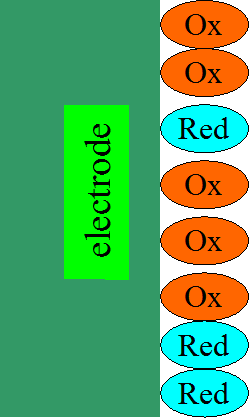
The current density is
| \( \displaystyle i=-nF\frac{d\Gamma_{\text{R}}}{dt}=nF\frac{d\Gamma_{\text{O}}}{dt} \) | (8.34) |
|---|
\( \Gamma_{\text{R}} \) and \( \Gamma_{\text{O}} \) are surface concentrations of reduced and
oxidized species, mol cm-2. Additionally, it is assumed
that the molecules do not dissolve from the surface, but at all times it holds that \( \Gamma_{\text{R}}(t)+\Gamma_{\text{O}}(t)=\Gamma_{\text{max}} \). A characteristic feature of the system is that when the electrode is
set to an arbitrary potential, the surface concentrations become such that the Nernst
equation always holds, i.e. every steady state is an equilibrium state at the
same time.
| \( \displaystyle\left(\frac{\Gamma_{\text{O}}}{\Gamma_{\text{R}}}\right)_{eq}=\theta_{eq}=\text{exp}\left[\frac{nF}{RT}(E_{eq}-E^0)\right] \) | (8.35) |
|---|
Analogously to Equation (8.18), a linearized current-voltage equation is expressed as
| \( \displaystyle\overline{\eta}(s)=\frac{RT}{nF}\left(\frac{\overline{i}(s)}{i_0}-\frac{\overline{\Gamma}_{\text{R}}(s)}{{\Gamma}_{\text{R},eq}}+\frac{\overline{\Gamma}_{\text{O}}(s)}{{\Gamma}_{\text{O},eq}}\right) \) | (8.36) |
|---|
The surface concentrations in the Laplace domain can be obtained directly from Equation (8.34):
| \( \displaystyle\overline{i}(s)=-nF(s\overline{\Gamma}_{\text{R}}(s)-\Gamma_{\text{R}, eq})=nF(s\overline{\Gamma}_{\text{O}}(s)-\Gamma_{\text{O}, eq}) \) |
(8.37) |
| \( \displaystyle
\frac{\overline{\Gamma}_{\text{R}}(s)}{{\Gamma}_{\text{R}},eq}=\frac{1}{s}-\frac{\overline{i}(s)}{nF\Gamma_{\text{R},eq}}\frac{1}{s}
\) ; \(
\displaystyle\frac{\overline{\Gamma}_{\text{O}}(s)}{{\Gamma}_{\text{O},eq}}=\frac{1}{s}+\frac{\overline{i}(s)}{nF\Gamma_{\text{O},eq}}\frac{1}{s}
\) |
(8.38) |
|---|
Substitution into Equation (8.36) gives
| \( \displaystyle Z=\frac{RT}{nFAi_0}+\frac{RT}{n^2F^2A}\left(\frac{1}{\Gamma_{\text{R},eq}}+\frac{1}{\Gamma_{\text{O},eq}}\right)\frac{1}{j\omega}=R_{ct}+\frac{1}{j\omega C} \) |
(8.39) |
|---|
The immobilized layer is modeled in impedance measurements as a combination of a resistor and capacitor in series, which is displayed as a semicircle on the admittance plot. The surface concentrations at equilibrium, \( \Gamma \)R,eq and \( \Gamma \)O,eq, can be determined using the Nernst equation and mass balance:
| \( \displaystyle\Gamma_{\text{O,}eq}=\Gamma_{\text{max}}\frac{\theta}{1+\theta} \) ; \( \Gamma_{\text{R,}eq}=\Gamma_{\text{max}}\frac{1}{1+\theta} \) |
(8.40) |
|---|
Now the quantity i0 can hardly be called exchange current density because it depends on the potential:
| \( \displaystyle i_0=nFk^0(\Gamma_{\text{R,}eq})^{1-\alpha}(\Gamma_{\text{O,}eq})^\alpha=nFAk^0\Gamma_{\text{max}}\frac{\theta^\alpha}{1+\theta} \) | (8.41) |
|---|
The unit for rate constant k0 is in this case s-1. The charge transfer resistance and capacitance are expressed as
| \( \displaystyle R_{ct}=\frac{RT}{n^2F^2A\Gamma_{\text{max}}k^0}\frac{\theta^\alpha}{1+\theta} \) |
(8.42) |
| \( \displaystyle\frac{1}{C}=\frac{RT}{n^2F^2A\Gamma_{\text{max}}}\frac{(1+\theta)^2}{\theta} \) |
(8.43) |
|---|
These
quantities as a function of potential without the constants are shown in Figure 8.14.
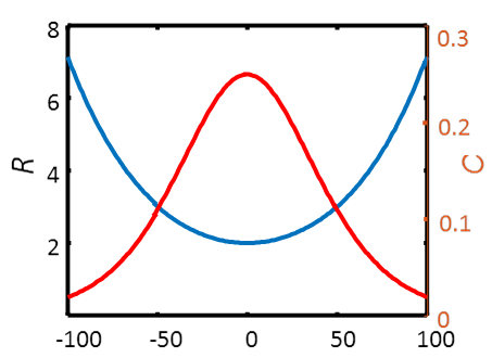
It is worth noting the high value of capacitance. A typical value for \( \Gamma \)max is 10-9 mol cm-2. If we substitute this value into the equation, the maximum capacitance becomes approximately 1 mF cm-2. The surface area of a porous material is high, and it is therefore possible to construct superconductors using immobilized redox species. The charge transfer resistance is also higher than usual. Assuming values \( \Gamma \)max = 10-9 mol cm-2 and k0 = 1 s-1, the order of magnitude of the maximum value of Rct will become 100 \( \Omega \) cm2.
Let us take a look at a model, which is a bit more realistic. In this model, a metal cation M+z is first adsorbed on the surface of the electrode and then reduced to a metal. The current density is
| \( \displaystyle\frac{i}{nF}=-k_c\Gamma_{\text{M}}=-k^0e^{-\alpha f(E-E^{0'})}\Gamma_{\text{M}} \) | (8.44) |
|---|
where n = z,
and the subscript ’c’ of kc denotes cathode process
and thus current is negative. The surface concentration of the cation \( \Gamma \)M can be expressed in terms of maximum surface
concentration and surface coverage \( \varphi \)*, \( \Gamma \)M = \( \Gamma \)max
\( \varphi \). The mass balance of the adsorbed cation is
| \( \displaystyle\frac{\partial\varphi}{\partial t}=\frac{i}{nF\Gamma_{\text{max}}}+k_ac_{\text{M}}^s(1-\varphi)-k_d\varphi=\frac{i}{nF\Gamma_{\text{max}}}+k_ac_{\text{M}}^s-(k_ac_{\text{M}}^s+k_d)\varphi \) | (8.45) |
|---|
where ka
and kd are adsorption and
desorption rate constants. It is therefore assumed that the adsorption is of a Langmuir
type. Let us simplify the expression by ignoring concentration polarization and
keeping solution concentration, \( c_{\text{M}}^s=c_0 \), constant, which means
that adsorption is the rate-limiting step. At a steady state, \( \partial\varphi/\partial t=0 \), and therefore
| \( \displaystyle\varphi_{ss}=\frac{i_{ss}/nF\Gamma_{\text{max}}+k_ac_0}{k_ac_0+k_d} \) | (8.46) |
|---|
The subscript ’ss’ denotes steady state. Linearizing Equation (8.44) and
transforming it to the Laplace domain gives
| \( \displaystyle\frac{\Delta\overline{i}(s)}{nF}=-k_c\Gamma_{\text{max}}(\Delta\overline\varphi(s)-\alpha f\varphi_{ss}\Delta\overline{E}(s)) \) | (8.47) |
|---|
Equation (8.45) is linear to begin with, so after
Laplace transformation we have
| \( \displaystyle s\Delta\overline{\varphi}(s)=\frac{\Delta\overline{i}(s)}{nF\Gamma_{\text{max}}}+\frac{k_ac_0}{s}-(k_ac_0+k_d)\Delta\overline\varphi(s) \) |
(8.48) |
| \( \displaystyle \Rightarrow
\Delta\overline{\varphi}(s)=\frac{\Delta\overline{i}(s)}{nF\Gamma_{\text{max}}(s+k_ac_0+k_d)}+\frac{k_ac_0}{s(s+k_ac_0+k_d)}
\) |
(8.49) |
|---|
| \( \displaystyle\frac{1}{nFA\Gamma_{\text{max}}}=-k_c\left(\frac{1}{nFA\Gamma_{\text{max}}(j\omega+k_ac_0+k_d)}-\frac{\alpha nF}{RT}\varphi_{ss}Z\right) \) | (8.50) |
|---|
Simplifying the expression gives
| \( \displaystyle Z=\frac{RT}{\alpha n^2F^2A\Gamma_{\text{max}}\varphi_{ss}}\left[\frac{1}{k_c}+\frac{1}{j\omega+k_ac_0+k_d}\right] \) | (8.51) |
|---|
The first term of Equation (8.51) is not
dependent on frequency, and thus it represents the charge transfer resistance. The
second term is a combination of two elements, and after giving it some thought,
it becomes evident that the term represents the parallel combination of a capacitor and a resistor. The equivalence circuit becomes complete when the double layer
capacitance, which is always present, is added in parallel with this faradaic
impedance, and we obtain the equivalent circuit and impedance plot displayed in
Figure 8.15.
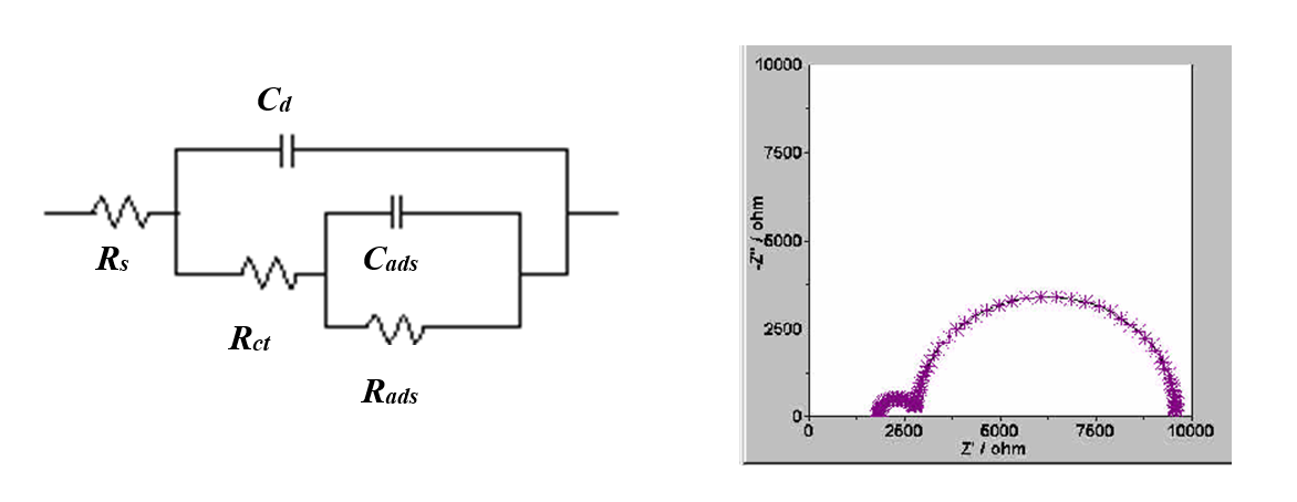
Figure 8.15. Equivalent circuit and impedance plot for an electrode reaction with an adsorption step.
Substituting jss into Equation (8.51), which we obtain using Equations (8.44) and (8.46):
| \( \displaystyle\varphi_{ss}=\frac{k_ac_0}{k_ac_0+k_d+k_c} \) | (8.51) |
|---|
Let us find the final expressions for Rct, Rads and Cads:
| \( \displaystyle R_{ct}=\frac{RT}{\alpha n^2F^2A\Gamma_{\text{max}}k_ac_0}\left(1+\frac{k_ac_0+k_d}{k_c}\right) \) |
(8.52) |
|---|---|
| \( \displaystyle R_{ads}=\frac{RT}{\alpha n^2F^2A\Gamma_{\text{max}}k_ac_0}\left(1+\frac{k_c}{k_ac_0+k_d}\right) \) |
(8.53) |
| \( \displaystyle C_{ads}=\frac{\alpha n^2F^2A\Gamma_{\text{max}}k_ac_0}{RT(k_ac_0+k_d+k_c)} \) |
(8.54) |
Values for physical parameters can be
determined as follows:
| \( \displaystyle\frac{R_{ct}}{R_{ads}}=\frac{k_ac_0+k_d}{k_c} \) |
(8.55) |
| \( \displaystyle R_{ads}C_{ads}=\frac{1}{k_ac_0+k_d} \) |
(8.56) |
| \( \displaystyle R_{ct}C_{ads}=1/k_c \) | (8.57) |
|---|
The impedance method therefore gives the value of the electrochemical rate constant explicitly, but finding the values of adsorption and desorption constants requires measurements at varying solution concentrations c0.
We have now shown that adsorption is observed as capacitance in impedance measurements. The derivation of impedance for more complicated mechanisms is, in principle, as simple as this; the only difference is that the mathematical treatment required is more extensive. The study of more complicated mechanisms is outside of the scope of this book. However, it is worth noting that even the previous example would be hopelessly difficult to study using other transient methods, and an analytical solution to the problem would not be possible.
* The symbol for surface coverage is usually \( \theta \), but we have already reserved it for the quantity exp[(nF)/(RT)(E - E0’)].
8.5. Other diffusion elements
The Warburg element is a result of a semi-infinite
diffusion field, in which the boundary condition is a finite concentration at
an infinite distance from the electrode surface. Usually, however, instead of
this boundary condition, the concentration is defined at the distance \( \delta \), which can be, e.g. the thickness of a
membrane or an unstirred layer (see Section 7.2) Applying the boundary condition\( c_{\text{R}}(\delta)=c_{\text{R},0} \), the surface
concentration in the Laplace domain becomes
| \( \displaystyle\overline{c}_{\text{R}}^s=\frac{c_{\text{R,0}}}{s}-\frac{\overline{i}(s)}{nF\sqrt{D_{\text{R}}}}\frac{\tanh\left(\delta\sqrt{s/D_{\text{R}}}\right)}{\sqrt{s}} \) | (8.58) |
|---|
For the species ’O’, the expression becomes
respectively
| \( \displaystyle\overline{c}_{\text{O}}^s=\frac{c_{\text{O,0}}}{s}+\frac{\overline{i}(s)}{nF\sqrt{D_{\text{O}}}}\frac{\tanh\left(\delta\sqrt{s/D_{\text{O}}}\right)}{\sqrt{s}} \) | (8.59) |
|---|
Instead of the Warburg element, the diffusion impedance consists of two tanh elements.
If there is an insulating layer through which current does not flow at the distance \( \delta \), one must use the boundary condition| \(\displaystyle\left(\frac{\partial c_k}{\partial x}\right)_{x=\delta}=0 \) ; k = R,O |
(8.60) |
|---|
In this case, a hyperbolic tangent is replaced
by a hyperbolic cotangent:
| \( \displaystyle\overline{c}_k^s=\frac{c_{k,0}}{s}\mp\frac{\overline{i}(s)}{nF\sqrt{D_k}}\frac{\coth\left(\delta\sqrt{s/D_k}\right)}{\sqrt{s}} \) ; k = R,O | (8.61) |
|---|
The minus sign is for the species ’R’ and the
plus sign for the species ’O’. Impedance plots of various diffusion elements
have been compared in Figure 8.16, and it becomes evident that there are
differences only at very low frequencies
f < 1 Hz. From this, we obtain a diagnostic criterion, when the
thickness of the finite diffusion layer needs to be taken into account:
| \( \displaystyle\frac{\delta}{\sqrt{D}}\sqrt{f}<1 \) | (8.62) |
|---|
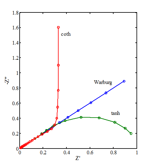
Figure 8.16. Diffusion elements tanh and coth compared to Warburg element. f = 0,1 ... 1000 Hz, \( \delta \)/√D = 1.
A typical value for the diffusion coefficient in water solution is 10-5 cm2s-1. If the lowest measurement frequency is 1 Hz, the diffusion layer has to be thinner than ca. 30 \( \mu \)m in order to observe differences compared to the Warburg element. If f = 0.1 Hz, the observed d increases to 100 \( \mu \)m. In practice, the use of tanh and coth elements is not common. At the boundary \( \delta\sqrt{f/D} \rightarrow0 \), a tanh element reduces to a resistor and coth element to a capacitor.
In the symmetrical thin layer cell in Figure 8.17, the following boundary condition holds:| \(\displaystyle \left(\frac{\partial c_k}{\partial x}\right)_{x=0}= \left(\frac{\partial c_k}{\partial x}\right)_{x=\delta} \) | (8.63) |
|---|
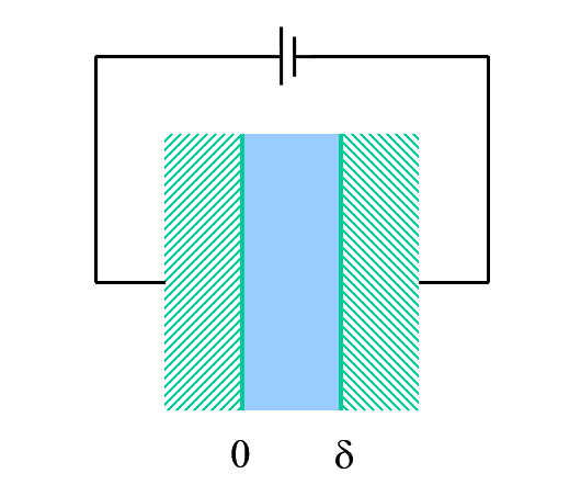
Thus the diffusion impedance is expressed as
| \( \displaystyle Z_{\text{diff}}=\frac{RT}{n^2F^2Ac_{k,0}}\frac{\tanh\left(\frac{1}{2}\delta\sqrt{j\omega/D_k}\right)}{\sqrt{j\omega}} \) | (8.64) |
|---|
Electrodes
with micrometer-sized dimensions are called (ultra) microelectrodes. The
diffusion field around these electrodes is almost spherical as shown in Figure 8.18.
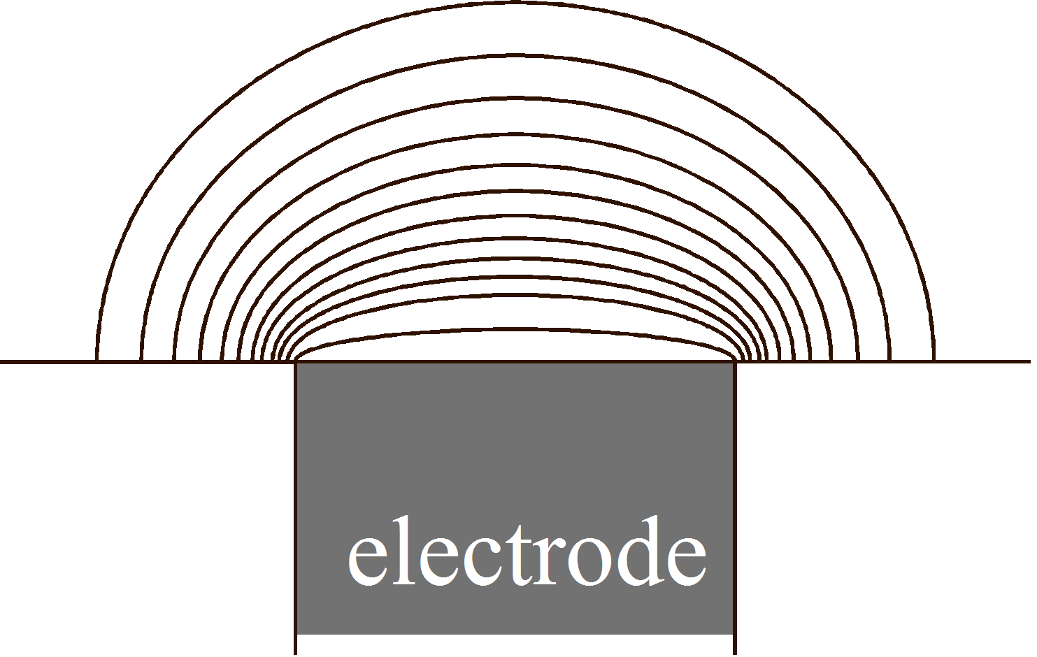
To be exact, the diffusion equation should be solved in cylindrical
coordinates, but in this case, the solution would contain modified Bessel
functions, which are not very illustrative.[1] We are satisfied with an approximation and use spherical coordinates. Now
Fick’s 2nd law becomes
| \( \displaystyle\frac{\partial c_k}{\partial t}=D_k\left[\frac{\partial^2c_k}{\partial r^2}+\frac{2}{r}\frac{\partial c_k}{\partial r}\right] \) | (8.65) |
|---|
The solution for the equation in the semi-infine diffusion field is
| \( \displaystyle\overline{c}_k=\frac{c_k^b}{s}+\frac{A(s)}{r}e^{-\lambda_kr} \) ; \( \displaystyle\lambda_k=\sqrt{\frac{s}{D_k}} \) |
(8.66) |
|---|
The current boundary condition for the species’R’ is expressed as
| \( \displaystyle D_{\text{R}}\left(\frac{\partial\overline{c}_{\text{R}}}{\partial r}\right)_{r=a}=\frac{\overline{i}(s)}{nF}=-\sqrt{D_{\text{R}}}\frac{A(s)}{a}e^{-\lambda_{\text{R}}a}\left(\sqrt{s}+\frac{\sqrt{D_{\text{R}}}}{a}\right) \) | (8.67) |
|---|
where a
is the radius of an electrode. The concentration on a sphere with a radius a is
| \( \displaystyle\overline{c}_{\text{R}}^s=\frac{c_{\text{R},0}}{s}-\frac{\overline{i}(s)}{nF\sqrt{D_{\text{R}}}}\frac{1}{\sqrt{s}+\sqrt{D_{\text{R}}}/a} \) | (8.68) |
|---|
Thus the diffusion impedance is
| \(\displaystyle Z_{\text{diff,}k}=\frac{RT}{n^2F^2Ac_{k,0}\sqrt{D_k}}\frac{1}{\sqrt{j\omega}+b} \) ; \( b=\frac{\sqrt{D_k}}{a} \) |
(8.69) |
|---|
The form \( (\sqrt{j\omega}+b)^{-1} \) corresponds to the parallel combination of Warburg element and a resistor (Figure 8.19). The graph of impedance is an arc of a circle \( Z'^2+Z''^2=Z'-Z'' \).
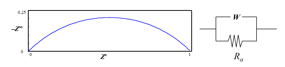
Figure 8.19. Diffusion impedance in spherical symmetry, b = 1.
If
the electrode reaction is coupled with a homogenous reaction, e.g. according to
the EC mechanism:
R – ne– \(\ce{ <=>[\ce{k(f)}][\ce{k(b)}] }\) O \(\ce{ ->[\ce{k(H)}] }\) products
where kH is the rate constant of a homogenous reaction, the solution for the species ’R’ is as before, i.e. Equation (7.7), but the diffusion equation of species ‘O’ becomes
| \( \displaystyle\frac{\partial c_{\text{O}}}{\partial t}=D_{\text{O}}\frac{\partial^2 c_{\text{O}}}{\partial x^2}-k_{\text{H}}c_{\text{O}} \) | (8.70) |
|---|
After taking the Laplace transform, the
solution is
| \( \displaystyle\overline{c}_{\text{O}}^s=\frac{c_{\text{O},0}}{s+k_{\text{H}}}+\frac{\overline{i}(s)}{nF\sqrt{D_{\text{O}}}}\frac{1}{\sqrt{s+k_{\text{H}}}} \) | (8.71) |
|---|
Thus it is evedent that the diffusion impedance of the species ’O’ is expressed as \( (j\omega+k_{\text{H}})^{-1/2} \), which is called the Gerischer impedance. The Gerisher impedance simulated with three different values of rate constants of a homogenous reaction are shown in Figure 8.20. Unlike in cyclic voltammetry, where small values of kH are more easily determined, the impedance technique tends to give higher values of kH. The impedance curve intersects the real axis at \( k_{\text{H}}^{-1/2} \). With small values of the rate constant of a homogenous reaction, the Gerischer impedance is identical to the Warburg impedance. Note that the shape of the Gerischer impedance resembles that of the tanh element presented in the previous section, which was a result of diffusion in a restricted space. If there is variation in the measurement data, it is crucial to know beforehand which processes are taking place in the system because otherwise a seemingly good fit into the equivalent circuit gives a misleading result. In practice, just like in the case of tanh and coth elements, the use of the Gerischer impedance is not common.
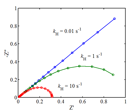
[1] The exact solution by Fleischmann and Pons can be found in J. Electroanal. Chem. 250 (1988) 277-283.
8.6. Corrosion
Impedance spectroscopy is also a good method for corrosion research. The typical corrosion reactions in acidic and basic
solutions are described in Section 6.5.4. Dissolution of a metal can formally
be written according to the Tafel equation:
| \(\displaystyle i_{\text{corr}}=i_{0,a}\left[e^{\alpha_anf(E_{\text{corr}}-E_a^0)}-e^{-\beta_anf(E_{\text{corr}}-E_a^0)}\right] \) |
(8.72) |
|---|
where i0,a is the exchange current density of the anode reaction, \( \alpha \)a and \( \beta \)a charge transfer coefficients, Ea0 equilibrium potential, and Ecorr corrosion potential of an electrode. If the cathode reaction is for example, hydrogen evolution, it can be considered irreversible, and
| \(\displaystyle i_{\text{corr}}=i_{0,c}e^{-\beta_cnf(E_{\text{corr}}-E_c^0)} \) |
(8.73) |
|---|
The quantities in Equation (8.73) correspond to those in Equation (8.72). The corrosion potential settles itself between the equilibrium potentials: \( E_c^0 < E_{\text{corr}} < E_a^0 \). If all variables in these equations are known based on, for example Tafel slopes, the corrosion potential can be solved because the anode and cathode reaction cancel each other out. If the equilibrium potentials are sufficiently far from one another, the inverse anodic reaction can be neglected and we have an expression derived by Stern and Geary for zinc dissolution with simultaneous hydrogen evolution [1]:
| \(\displaystyle i_{\text{corr}}=i_{0,a}e^{\alpha_anf(E_{\text{corr}}-E_a^0)}=i_{0,c}e^{-\beta_anf(E_{\text{corr}}-E_c^0)} \) | (8.74) |
|---|
Interpreting icorr as an exchange current of the corrosion reaction, the current-overpotential equation becomes
| \(\displaystyle i=i_{\text{corr}}(e^{\alpha_anf\eta}-e^{-\beta_cnf\eta}) \) | (8.75) |
|---|
where \( \eta \) = E - Ecorr. Hence the expressions for the currents can be linearized in the vicinity of \( \eta \) = 0:
| \( \displaystyle\frac{i}{i_{\text{corr}}}=1+\alpha_anf\eta-1+\beta_cnf\eta=(\alpha_a+\beta_c)nf\eta \Rightarrow \frac{i}{i_{\text{corr}}}=(\alpha_a+\beta_c)\frac{nF}{RT}R_p \) | (8.76) |
|---|
where Rp is polarization resistance. Corrosion current is easy to determine using the value of Rp, which is obtained from the diameter of the semicircle in the impedance plot. Often in corrosion literature the charge transfer coefficients are expressed in term of Tafel slopes (see Section 6.2.2), but more importantly, \( \alpha \)a + \( \beta \)c ≠ 1.
Corrosion
can be studied by setting the electrode at such a high anodic potential that
metal begins to dissolve. Then current naturally flows across the electrode and
the analysis becomes more complicated. Consider a two step mechanism, where
metal first forms a univalent cation M+, which remains adsorbed at
the surface. In the second step, the univalent cation is oxidized to a soluble
bivalent cation M2+.
| M \(\ce{ -> }\) M+* + e– | \( k_1=k_1^0e^{b_1\eta} \) |
|---|---|
| M+* \(\ce{ -> }\) M2+(aq) + e– | \( k_2=k_2^0e^{b_1\eta} \) |
k1 and k2 are the reaction rate constants of the steps and b1,2 = \( \beta \)1,2×F/RT.
Again, let the symbol \( \varphi \) denote the surface coverage of the adsorbed cation. Current is the sum of the first and second steps:
| \( \displaystyle\frac{i}{F\Gamma_{\text{max}}} =k_1(1-\varphi)+k_2\varphi \) | (8.77) |
|---|
The term k1(1 - \( \varphi \)) describes the process in which the metal is
only dissolved from the free surface. The mass balance for the adsorbed species
M+* is
| \( \displaystyle\frac{d\varphi}{dt} =k_1(1-\varphi)+k_2\varphi \) | (8.78) |
|---|
Surface coverage thus changes only due to
electrochemical reactions. In a steady state, d\( \varphi \)/dt = 0, and \( \varphi \)ss =k1/(k1 + k2).
After linearization and taking the Laplace transform of Equation (8.77):
| \( \displaystyle\frac{\Delta\overline{i}}{F\Gamma_{\text{max}}}=(1-\varphi_{ss})\Delta\overline{k}_1(s)-k_1\Delta\overline{\varphi}(s)+\varphi_{ss}\Delta\overline{k}_2(s)+k_2\Delta\overline{\varphi}(s)=[(1-\varphi_{ss})b_1k_1+\varphi_{ss}b_2k_2]\Delta\overline{\eta}(s)-(k_1-k_2)\Delta\overline{\varphi}(s) \) | (8.79) |
|---|
Using the expression for \( \varphi \)ss and after some algebra, we obtain
| \( \displaystyle \frac{\Delta\overline{i}(s)}{F\Gamma_{\text{max}}\Delta\overline{\eta}(s)}=\frac{(b_1+b_2)k_1k_2}{k_1+k_2}-(k_1-k_2)\frac{\Delta\overline{\varphi}(s)}{\Delta\overline{\eta}(s)} \) | (8.80) |
|---|
After linearization and taking the Laplace transform of Equation (8.76):
| \(\displaystyle s\Delta\overline{\varphi}(s)=(1-\varphi_{ss})\Delta\overline{k}_1(s)-k_1\Delta\overline{\varphi}(s)-\varphi_{ss}\Delta\overline{k}_2(s)-k_2\Delta\overline{\varphi}(s)=[(1-\varphi_{ss})b_1k_1-\varphi_{ss}b_2k_2]\Delta\overline{\eta}(s)-(k_1+k_2)\Delta\overline{\varphi}(s) \) |
(8.81) |
| \(\displaystyle \Rightarrow (s+k_1+k_2)\frac{\Delta\overline{\varphi}(s)}{\Delta\overline{\eta}(s)} =\frac{(b_1-b_2)k_1k_2}{k_1+k_2} \) | (8.82) |
|---|
Combining Equations (8.80) and (8.82) the
corrosion impedance is
| \( \displaystyle Z_{\text{corr}}^{-1}=FA\Gamma_{\text{max}}\frac{k_1k_2}{k_1+k_2}\left[b_1+b_2-\frac{(b_1+b_2)(k_1-k_2)}{k_1+k_2+j\omega}\right] \) | (8.83) |
|---|
The brackets include two terms, which means parallel elements because we are
dealing with admittance. The first term is independent of the frequency: hence it is a resistor. The reciprocal of the second term, i.e. its impedance form is, a sum of a frequency-independent term and another term that is directly
proportional to jω. This sum is therefore a series combination of a resistor
and an inductor. The total impedance is therefore
| \( \displaystyle Z_{\text{corr}}^{-1}=\frac{1}{R_t}+\frac{1}{R_{ad}+j\omega L_{ad}} \) | (8.84) |
|---|
The equivalent circuit and the capacitance of
the electrode as well as a simulated impedance plot are shown in Figure 8.21. The
expressions for the elements can be written as
| \( \displaystyle R_t=\frac{1/k_1+1/k_2}{FA\Gamma_{\text{max}}(b_1+b_2)} \) |
(8.85) |
|---|---|
| \(\displaystyle R_{ad}=-\frac{(1/k_1+1/k_2)(k_1+k_2)}{FA\Gamma_{\text{max}}(b_1-b_2)(k_1-k_2)} \) |
(8.86) |
| \(\displaystyle L_{ad}=-\frac{(1/k_1+1/k_2)\Gamma_{\text{max}}}{FA\Gamma_{\text{max}}(b_1-b_2)(k_1-k_2)} \) |
(8.87) |
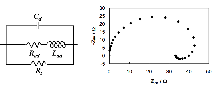
Figure 8.21. Equivalent circuit of corrosion impedance and a simulated impedance plot, Rt = 50 W, Rad = 100 \( \omega \), Lad = 0,01 H and Cd = 0,5 \( \mu \)F.
It is remarkable that Rad and Lad can have negative values, but they must have the same sign because
| \(\displaystyle \frac{L_{ad}}{R_{ad}}=\frac{1}{k_1+k_2} \) | (8.88) |
|---|
Reaction rate constants k1 and k2 can be determined from the values of the elements as follows:
| \( \displaystyle k_1=\frac{R_{ad}}{2L_{ad}}\left(1-\frac{b_1+b_2}{b_1-b_2}\frac{R_t}{R_{ad}}\right) \) |
(8.89) |
| \(\displaystyle k_2=\frac{R_{ad}}{2L_{ad}}\left(1+\frac{b_1+b_2}{b_1-b_2}\frac{R_t}{R_{ad}}\right) \) | (8.90) |
|---|
The factors b1 and b2 must be determined separately, e.g. from Tafel slopes. If they are equal, the impedance is simplified to Rt (see Equation (9.92)).
The characteristic feature of corrosion impedance is the inductive loop below the real axis at low frequencies. If there are several adsorption steps, each of them will give its own loop. At high frequencies, an inductive loop below the real axis is sometimes seen, but it is due to the wires connecting the cell and the measurement apparatus (potentiostat). It can be modeled as an inductor in series with the solution resistance.
8.7. Dispersion of time constants
One of the key concepts in the impedance analysis is the time constant. As we have seen earlier, a resistor and a capacitor are always paired, and when impedance is determined, the result includes terms with the product RC. The dimension of this product is actually a second, and thus the constant is defined as \( \tau \) = RC. The dimension of the quotient L/R is also a second, but such terms do not exist. We therefore usually say that the circuit in Figure 8.4 is characterized by one time constant, but the circuit in Figure 8.15 has two time constants. The number of the time constants is therefore equal to the number of semicircles in the impedance plot. In the combination of R and C in series, the semicircle is seen in the admittance plot. If the time constants are almost equal in magnitude, it can be difficult to distinguish between them.
In
practice, the semicircles observed are rarely perfect, but they seem to be
flattened in the imaginary direction. The phenomenon is taken into account by replacing C with a constant phase element (CPE), for which the admittance is
| \( Y=Y_0(j\omega)^\alpha \) |
(8.91) |
|---|
The range of the factor a, i.e. the frequency in Equation (8.88) is in
theory [-1,1], but in practice [0,1]. If \( \alpha \) =
0, CPE is a resistor and Y0 = 1/R. When \( \alpha \) = 0.5, CPE corresponds to the Warburg element,
and \( Y_0=\sqrt2/\sigma \) (see (8.22)). If \( \alpha \) = 1, CPE is a capacitor and Y0 = C. If \( \alpha \) = -1, CPE is an inductor, and Y0
= L-1. The name constant phase element derives from the fact that the angle
of the impedance vector is constant independent of frequency:
| \( j^\alpha=(e^{j \pi/2})^\alpha=e^{j \alpha \pi/2}=\cos(\alpha \pi/2)+j\sin(\alpha \pi/2) \) | (8.92) |
|---|
The flattened semicircle in the impedance plot is obtained when \( \alpha \) < 1. Simulated R-CPE circuits with three different values of a are shown in Figure 8.22. The figure illustrates that the smaller \( \alpha \), the more the semicircle is flattened.
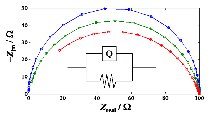
Figure 8.22. Impedance plots of a constant phase element and a resistor in parallel with values of \( \alpha \) = 1, 0.9 and 0.8; R = 100 \( \Omega \) and Y0 = 10-7 \( \Omega \)-1. The symbol Q describes the CPE in the fitting software.
In practice, the angle of 45 degrees, which corresponds to the Warburg element, is not reached either, but it remains smaller. In this case, the Warburg element is replaced by CPE, where \( \alpha \) < 0.5. Even though it is mathematically possible to take into account the descent of the semicircle and the inclination of the Warburg line using CPE, for every CPE there will be one parameter more in the mathematical treatment. Because of this, it is harder for the iteration to converge, and thus the model may produce erroneous results.
Naturally,
the next question we want to ask is about the physical source or interpretation of
CPE. The answer lies in the heterogeneity of the electrode surface. First, the
surface is far from being completely smooth. Instead, it is rough at least at
a molecular level, and usually also at a micrometer level. Second, the
electrode surface is not chemically completely heterogeneous either, but it may
contain oxidized passive domains or very active areas, for example at the boundaries
of crystal surfaces. Because of this, the reaction rate constant and the
corresponding charge transfer resistance do not have one single value, but a
distribution of values at different points on the surfaces. As a result, the
circuit does not have one single time constant, but rather a distribution of time
constants. The equivalent circuit of the case is illustrated in Figure 8.23.
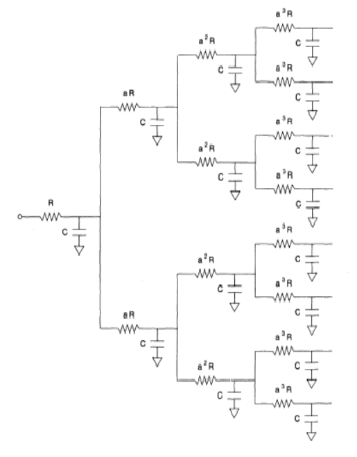
The
diffusion element is affected by the surface roughness in a different manner. If
the surface of the electrode were completely smooth, the concentration at a
given distance from the surface would be constant. But if the surface is rough,
there will be equi-concentration planes near the surface of the electrode. Consider Figure 8.24. At a molecular level, diffusion can be seen as Brownian
motion. The probability of our test particle hitting the surface of the
electrode during a time step Dt is greater at point B than at point A.
On the other hand, the average time for the particle to reach the surface is
shorter at point B than at point A. The total current
observed in experiments therefore provides information on the surface roughness with
respect to the average diffusion distance \( l \sim\sqrt{D\Delta t} \). This is seen
in the potential step experiments (Chapter 7) as the current does not decrease \( \sim t^{-1/2} \) but is a bit
more gradual, and also the inclination of the Warburg line is lower.
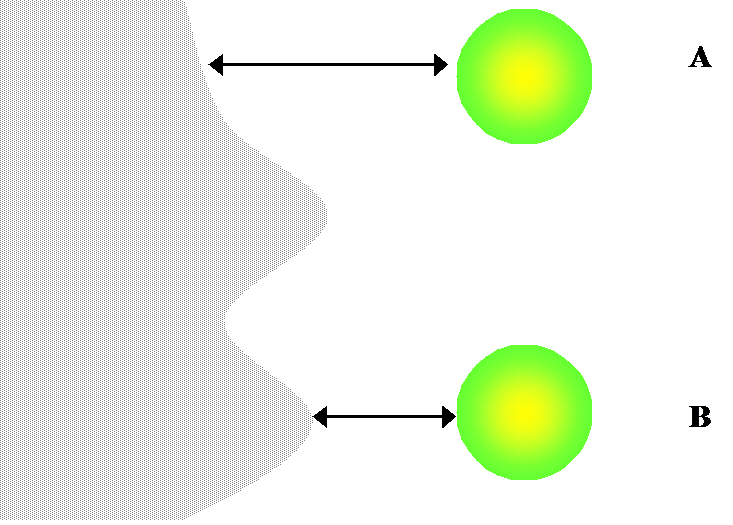
It is evident that the more heterogeneous the surface,
the lower the value of \( \alpha \). However, the
heterogeneity of the surface can be evaluated in a more analytical manner.
It has been suggested [1]
that the frequency exponential of the CPE \( \alpha \) and the fractal dimension DF
are related as
Looking at Equation (8.93) it is obvious that because the dimension of the euclidic surface is 2, \( \alpha \) is equal to 1. The fractal dimensions of physical surfaces are in the range 2.1-2.3, which means that the range of a is 0.77-0.91, which is exactly what we observe in measurements. At the frequency range of diffusion, the Warburg element is replaced by the CPE with \( \alpha \) < 0.5. In this case, the relation has been suggested to be [2]
From Equation (8.94) it is seen that if \( \alpha \) < 0.5, DF < 2. Because of this, it is a bit confusing that the same surface gives DF > 2 at the frequency range of CPE, and DF < 2 at the frequencies of diffusion. However, these different processes are observed at different ranges of frequencies. It is necessary to keep in mind that the fractal nature of the surface is not solely its roughness, but the fractals are required to be similar, which means that the shape of the surface must be replicated at all magnifications. In practice, this cannot be the case, but the characteristics of the surface must be repeated at least in four different orders of magnitude in order for the surface to be fractal. |
|---|
[1] T. Pajkossy, L. Nyikos, J. Electrochem. Soc. 133 (1986) 2061.
[2] A.P. Borosy, L. Nyikos, T, Pajkossy, Electrochim. Acta 36 (1990) 163.
8.8. Transmission lines
A transmission line is an alternative way to
describe charge transfer mechanisms. A schematic representation of a
transmission line is shown in Figure 8.25.

Figure 8.25. Simple transmission line.
The same transmission line can be drawn in an
electrically identical form, which enables the determination of the impedance
of the whole transmission line.
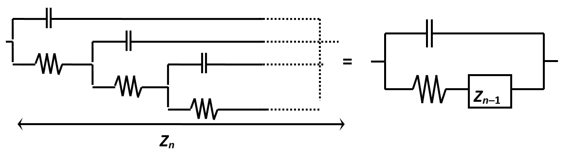
From the right-hand side of the scheme of Figure 8.26, the impedance can
be determined as follows:
| \( \displaystyle Z_n=\frac{1}{j\omega C+\frac{1}{R+Z_{n-1}}} \) | (8.95) |
|---|
Because of the infinite length of the transmission line, Zn = Zn-1 = Z, and Z can be solved:
| \( \displaystyle Z=\frac{R}{2}\left(\sqrt{1+\frac{4}{j\omega RC}-1}\right) \approx\sqrt{\frac{R}{j\omega C}} \) | (8.96) |
|---|
Equation (8.96) is of the form (j\( \omega \))-1/2, that is the Warburg impedance. The following is given without proof: If the length of the line is finite and the end of the line short-circuited, the line represents the tanh element. If the end of the line is open, it is the coth element, see Figure 8.16.
The
impedance plot of a porous membrane is a semicircle, which is a little difficult
to understand. If a pore in the membrane is modeled as a straight capillary
with a given surface charge density and filled with an electrolyte solution,
the following transmission line can be drawn, which originally describes an
electric conductor with finite conductivity:
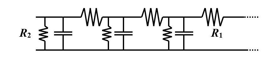
Figure 8.27. Transmission line of a conductor with a finite conductivity.
Analogously to Figure 8.26, this line can be redrawn as:
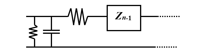
Figure 8.28. Reduced transmission line of Figure 8.27.
Again, the impedance can be solved assuming the
line infinite:
| \( \displaystyle\frac{1}{Z_n}=j\omega C+\frac{1}{R_2}+\frac{1}{R_1+Z_{n-1}} \Rightarrow Z=\frac{R_1}{2} \left(\sqrt{1+\frac{4}{R_1(1/R_2+j\omega C)}}-1\right) \) | (8.97) |
|---|
Taking into account that with small values of x,
\( \sqrt{1+x} \approx1+\frac{1}{2}x \) and
Equation (8.97) can be expressed as:
| \( \displaystyle Z \approx\frac{1}{1/R_2+j\omega C} \) | (8.98) |
|---|
This is the parallel combination of C and R2, which gives the desired semicircle [1].
[1] If you are wondering about the approximations or the conclusions drawn, it is easy to check the validity of them using any mathematical software (Matlab, Mapple, Mathematica) and realize that the impedance plots can be constructed even without approximations.
8.9. Kramers-Kronig transforms
The following criteria must hold in an impedance measurement:
1. Causality. The causality criterion means that the system response is only due to the perturbation applied, and does not contain contributions from spurious sources.
2. Linearity. The relation between the system perturbation and response is described by a set of linear differential laws.
3. Stability. The system must be stable in the sense that it returns to its original state after the perturbation is removed.
4. Finite-valued. Impedance must be finite at \( \omega \) → 0 and \( \omega \) → ∞, and must be a continuous and finite function at all frequencies.
Under
these conditions, a set of transforms between the real and imaginary components
are held, known as Kramers-Kronig transforms, the following two being the most
important of these:
| \( \displaystyle Z'(\omega)-Z'(\infty)=\frac{2}{\pi} \int_{0}^{\infty}{\frac{xZ''(x)-\omega Z''(\omega)}{x^2-\omega^2}} dx \) |
(8.99) |
| \( \displaystyle Z''(\omega)=-\frac{2}{\pi} \int_{0}^{\infty}{\frac{Z'(x)-Z'(\omega)}{x^2-\omega^2}} \) | (8.100) |
|---|
In Equations (8.99) and (8.100) x is an auxiliary variable (frequency). The transforms are solely mathematical and generic, and thus they do not contain any physical interpretations. In terms of impedance measurements, the fourth criterion is slightly problematic. At low frequencies, the impedance is controlled by mass transfer, i.e. diffusion. However, the Warburg and coth elements increase boundlessly when \( \omega \) approaches zero. We can avoid the problem when determining the integrals by using an equivalent circuit that gives the same result at the boundary. Consider, for example, the coth element. Figure 8.16 illustrates that at low frequencies, it corresponds to the combination of \( R+1/(j\omega C) \). The term xZ”(x) ≈ -x/(xC) = -1/C in the integral (8.99) is therefore a finite number. Respectively, for the Warburg element, the product \( \omega \)Z”(\( \omega \)) ~ \( \omega \)1/2 → 0, when \( \omega \) → 0.
Kramers-Kronig transform is usually integrated in the control and analysis software of a potentiostat, and there is no need for the user to know which algorithm is used for the mathematical treatment of the integral or how the boundary values of frequency are treated. As the transform is easily available in the software, it is useful to do the transform from time to time. For example, if the experimental conditions are such that the electrode is passivated easily, it is important to check that the stability criterion is still holding.
8.10. Similarities of the equivalent circuits
The challenge in the interpretation on the
impedance data is that the data may fit with more than one equivalent circuit.
It is therefore crucial for the researcher to know or make an educated guess
about the processes in the system. Three different circuits are presented in
Figure 8.29 that all give the same impedance plot; the values of the elements
are obviously not equal in different circuits.
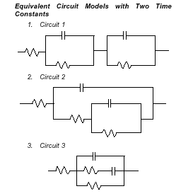
Figure 8.29. Three different equivalent circuits that give similar impedance.
The first circuit in Figure 8.29 could illustrate a membrane system. The two RC circuits would correspond to the surfaces of the membrane, and the resistor in front of the system would include all the ohmic resistance of the system. The second circuit is typical for an electrode, when the electrode reaction is accompanied by an adsorption step (see chapter 8.3.2 and Figure 8.15). The third circuit includes a series combination of a resistor and a capacitor, illustrating, for example, dipolar relaxation in the solid phase [1]. This circuit is therefore typical in the electrochemistry of the solid phase.
An alternative to the Randles circuit is shown in Figure 8.30.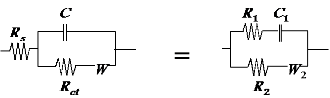
Figure 8.30. The circuit (right), which gives an identical impedance compared to the Randles circuit (left).
In corrosion research in particular it is necessary to be careful, because, as shown in Section 8.3.4, the elements may even have negative values. The loop below the real axis in Figure 8.21 can also be modeled using the parallel combination of a resistor and a negative capacitor.
[1] See, for example, J.R. Macdonald, Impedance Spectroscopy, John Wiley & Sons, New York 1987, s. 49.
8.11. Some remarks on the experimental arrangement of impedance measurements
The measurement of impedance using modern computer-controlled workstations is very fast and easy. The only responsibility of the operator is to make sure that the parameters in the experiment are reasonable. The amplitude of the input signal is not recommended to be greater than approximately 50 mV (peak-to-peak), in order to maintain the linearity of the system. The required frequency range usually depends on the system being examined. At low frequencies, the system is controlled by mass transfer, which is not necessarily interesting in the impedance measurements. In addition to this, the measurements at low frequencies last longer, as a result of which the instability of the system may pose a problem. On the other hand, at high frequencies, the connections of the cell and the potentiostat add to the perturbation. The connections of the electrode are observed as inductance in the series combination with the cell.
One of the most important parameters in terms of the quality of the measurement data is the integration time, i.e. how many measurement cycles are averaged in the mathematical treatment of the data. It is recommended to have at least 10 cycles; 5 is the absolute minimum. In some systems, it is possible to use what is known as multisine mode, in which the input signal consists of various frequencies at low frequencies in particular. The analysis is based on the Fourier transform, which separates the contribution of each frequency in the output signal. For some unknown reason, the impedance data obtained using the Fourier analysis may deviate from the ordinary impedance data, and a dummy connection, for example, must be used to make sure that the Fourier analysis is giving the correct data.
The fitting software is usually integrated into the measurement software, and the only task left for the operator is to find the equivalent circuit that fits the data. The greatest challenge, however, is the physical interpretation of the equivalent circuit. It is possible to improve the quality of the fit by adding elements to the circuit, but this kind of circuit lacks physical meaning because it fits any given data. Usually the software gives an error function \( \chi^2 \), which describes the sum of squares of the error. A general rule for an acceptable fitting of the equivalent circuit is \( \chi^2 \) < 10-4. Data points can be added in order to improve the convergence of the fit. In addition, the fitting software usually gives various alternatives for the weighting of the data. In practice, the best result is obtained using modulus weighting, in which the weight of the data point is proportional to the length of the impedance vector.
Finally, the importance of the design of the measurement cell has to be emphasized. The current distribution at the working electrode should be as even as possible. The area of the counter electrode should be greater than that of the working electrode because otherwise the impedance of the counter electrode is included in the data. The ohmic resistance between the working electrode and the counter electrode or between the working electrode and the reference electrode should not be too large in magnitude, or the potentiostat may not be able to control the measurement properly. In addition, the measurement should be repeated without the examined electroactive species in order to separate the factors caused by the geometry of the cell from the measurement data.
You can now test your conceptual knowledge by taking Quiz Chapter 8.
9. Electrochemical energy conversion
Versatile electrochemical energy conversion technologies are used for powering numerous electrical devices, ranging from small-scale consumer applications such as watches and mobile phones to electric vehicles and even to distributed energy systems. Furthermore, the need for energy conversion in society is increasing due to the transition from fossil fuel-based energy supply to renewable yet intermittent energy technologies. One of the challenges related to these new energy supply technologies is to ensure continuous availability of energy during low production periods. Renewable energy technologies therefore need to be supplemented with devices for short-term (peak shaving) and long-term energy storage, whereby energy is converted to other forms during peak productions periods. Moreover, transition is also going on in the mobile sector, with the adoption of electrical vehicles, e-bikes and other small-scale personal transportation devices. A plethora of energy conversion technologies have been introduced in the past few years but only few have achieved commercial maturity, or even a demonstration phase.
Batteries, flow batteries and fuel cells are galvanic devices that convert energy stored in chemical compounds directly into electricity via spontaneous electrochemical reactions. In batteries, chemicals generating electrical energy during electrochemical reduction and oxidation reaction are stored in the device. In primary batteries, the electrodes are consumed in irreversible electrochemical reactions, and they cannot be re-charged because of potentially hazardous side reactions. In secondary batteries, electrode materials participate in reversible reactions, and they have been designed to withstand several charging and discharging cycles.
In flow batteries, the reactants are fed into the electrochemical reactor from external reservoirs. The reactions are reversible at both electrodes. When re-charging the device, the direction of the reactant flow is reversed. The volume of the reservoirs therefore determines the duration of the charging- discharging cycle. Because of the external storage of the chemicals, flow batteries are easy to upscale. In a similar manner to flow batteries, in fuel cells, fuel (e.g. hydrogen or methanol) is fed to the anode from an external source. At the cathode, however, airborne oxygen serves as the oxidant.
In addition to galvanic cells, supercapacitors and electrolyzers are introduced in this chapter. Electrolyzers are electrolysis cells, a kind of reversed fuel cells that convert electrical energy in non-spontaneous reactions into the form of chemical bond energy. Electrochemical double layer supercapacitors are reminiscent of batteries but, instead of an electrochemical reaction, the energy storage is based on adsorption.
The characteristics and performance of all these devices is largely determined by the choice of cathode and anode materials, as well as by the electrolyte. However, engineering also plays an important role because of the various transport phenomena occurring in the cells.
From classical thermodynamics (see Chapter 1), we know that the Gibbs free energy provides the upper limit for chemical energy that can be converted into electrical energy
| \( W_{el}=\Delta G=\Delta H -T\Delta S=-nFE \) | (9.1) |
|---|
The open circuit voltage can be calculated if the Gibbs free energies of the electrode reactions or the standard electrochemical reduction potentials are known. However, the cell potential also depends on the temperature, pressure and concentrations of the reacting species:
| \( \displaystyle E^{eq}=-\left(\frac{\Delta H}{nF}-\frac{T\Delta S}{nF}\right)+\frac{RT}{nF}\ln\left(\frac{\Pi C_r}{\Pi C_p}\right) \) | (9.2) |
|---|
Electrical energy is generated when current is drawn from the cell. In this case, energy is also consumed in other processes, such as overcoming kinetic reaction barriers, in transport phenomena and ohmic losses, as described in Chapter 6. All these phenomena must be taken into account when determining the current-voltage characteristic of the cell.
| \( E=E^{eq}(T,P,c)-\eta_{act,a}-|\eta_{act,c}|-\eta_{diff,a}-|\eta_{diff,c}|-A \cdot i \cdot R \) | (9.3) |
|---|
A typical current-voltage response or a polarization curve of an alkaline cell is depicted in Figure 9.1. The cell potential therefore decreases when more current is drawn from the cell because of the various losses given in Equation (9.3). As for an electrolysis cell, these losses are added to the overall cell voltage, thereby increasing the voltage needed to run the conversion of electrical energy into chemical form.
| \( E=E^{eq}(T,P,c)+\eta_{act,a}+|\eta_{act,c}|+\eta_{diff,a}+|\eta_{diff,c}|+A \cdot i \cdot R \) | (9.4) |
|---|
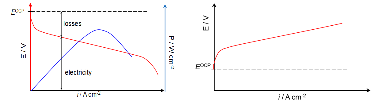
Figure 9.1. In a galvanic cell (left), overpotential and ohmic losses lower the applicable cell voltage, red curve; blue curve depicts the cell power. In an electrolysis cell (right), overpotential and ohmic losses increase the cell voltage needed to run a process accordingly.
9.1. Supercapacitors
Supercapacitors, also known as ultracapacitors, are electrochemical devices that utilize the double layer region of the potential window for short-term energy storage. In a sense, they are reminiscent of conventional capacitors, but the charge separation and electric field is created across the electrical double layers (Chapter 5) formed at the both electrodes (Figure 9.2), instead of dielectric material used in the conventional capacitors. These devices have two similar electrodes separated by an aqueous or organic electrolyte.
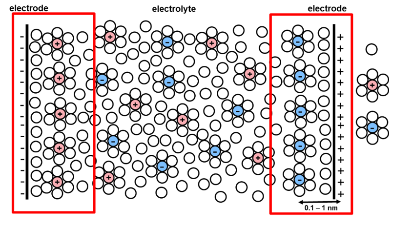
With supercapacitors, high energy density is achieved compared to conventional capacitors, which is based on two factors: First, combining porous 3D electrodes (in commercial devices made of activated carbon) and a liquid electrolyte (often TEABF4 in acetonitrile) results in a large surface area (see Equation (9.5)). Second, the distance between the electrode surface and the ions in the double layer region is very small, of an atomistic scale.
| \( \displaystyle C=\frac{Q}{U}=\varepsilon\frac{A}{d} \) | (9.5) |
|---|
Because the energy storage mechanism in supercapacitors is based on the formation of the double layer on the electrode-electrolyte interface, no electrochemical reactions take place. The energy can therefore be stored and released quickly, leading to high power density and minimal degradation of the materials. As a result, these devices can withstand hundreds of thousands of charge-discharge cycles and are suitable for high-power applications, e.g. storing mechanical energy when vehicles brake[1]. The downside is that the energy density is relatively low (compared to batteries) and the self-discharge rate is relatively high.
In order to increase the energy density, redox supercapacitors that utilize fast and reversible electrochemical surface reactions for the charge storage have been developed. These include MnOx and RuOx redox processes. Hybrid supercapacitors that combine electrodes with dissimilar storage principles are also being investigated. A combination of an electrode type used in the lithium-ion battery with an EDLC or redox electrode can be mentioned as an example of hybrid devices.
9.2. Primary batteries
Dozens of different primary battery chemistries have been developed, and batteries with various shapes are available for consumers, ranging from coin cells to cylindrical and prismatic ones. In wearable electronics, flexible thin batteries are often used, while in Internet of Things (IOT)- type applications small primary batteries often power the devices. The most common consumer batteries utilize zinc-manganese, zinc-air and lithium-ion chemistries. The major features of primary lithium-ion batteries are similar to those of secondary lithium-ion batteries, but they have a metallic lithium anode. These batteries have been designed for a single use and attempts to recharge then can lead to hazardous side reactions or even an explosion.
9.2.1 Zinc-Manganese chemistry: Lechlanché and alkaline battery
The alkaline battery is equivalent to the acidic Lechlanché battery or zinc-carbon battery, the discovery of which dates back approximately 150 years. Lechlanché batteries are still in use in a number of consumer and professional applications because they are affordable in price and easy to design to meet specific shape and capacity requirements. However, alkaline batteries are now the most popular primary batteries because they are more reliable than Lechlanché batteries and allow the high discharge currents required in portable consumer electronics. The capacity of alkaline batteries also stays relatively stable over a large range of currents and temperatures and they can be stored for relatively long periods.
The cell voltage of the zinc manganese chemistry is approximately 1.5 V. The structure of the Lechlanché battery with the aqueous solution of NH4Cl and ZnCl electrolyte is given on the left of Figure 9.3. In these batteries, MnO2 serves as the cathode material and Zn as the anode. The electrode reactions are:
Anode: Zn(s) + 2 OH−(aq) \(\ce{ \bond{->} }\) ZnO(s) + H2O(l) + 2e−
Cathode: 2 MnO2(s) + H2O(l) + 2e− \(\ce{ \bond{->} }\) Mn2O3(s) + 2 OH−(aq)
Overall: 2 Zn(s) + 2 MnO2(s) + H2O(l) \(\ce{ \bond{->} }\) MnOOH(s) + 2 ZnO(s)
In an alkaline battery, similar electrode materials are used (on the right of Figure 9.3), except that concentrated immobilized KOH is used as the electrolyte. Under these conditions, the following reactions take place:
Anode: Zn(s) \(\ce{ \bond{->} }\) Zn2+ (aq) + 2e−
Cathode: 2 MnO2(s) + 2 H2O + 2e− \(\ce{ \bond{->} }\) 2MnOOH (s) + 2 OH−(aq)
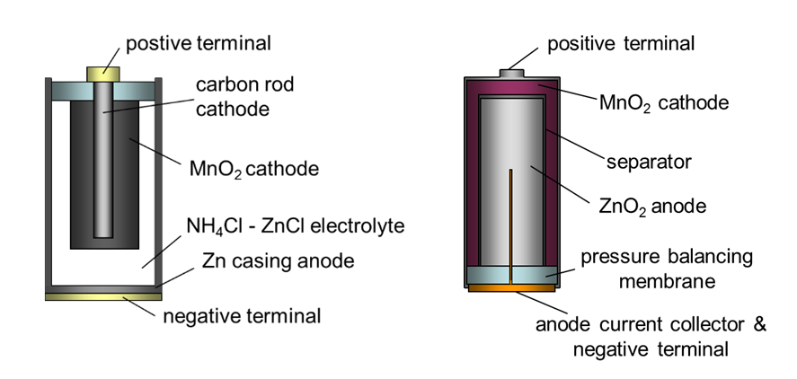
Figure 9.3. Sketch of a Leclanché (left) and an alkaline battery (right).
9.2.2 Zinc-air battery
A Zinc-air battery is introduced here as an example of batteries where one of the electrodes participating the reactions is replaced by an electrocatalyst (see Figure 9.4). Because of the compact structure of the air cathode, high energy densities are achieved with this primary battery. It is therefore suitable for continuous operation in applications requiring high performance at low investment costs. The applications extend from consumer hearing aids to industrial scale devices.
Because of the gelled alkaline KOH electrolyte, the anode reaction is similar to that in an alkaline battery. However, airborne oxygen reacts on the surface of the cathode producing hydroxyl ions. The resulting battery voltage is 1.2 V.
Anode Zn \(\ce{ \bond{->} }\) Zn2+ + 2e−
Zn2+ + 2OH− \(\ce{ \bond{->} }\) Zn(OH)2
Zn(OH)2 \(\ce{ \bond{->} }\) ZnO + H2O
Cathode ½ O2 + H2O + 2e− \(\ce{ \bond{->} }\) 2OH−
Overall Zn + ½O2 \(\ce{ \bond{->} }\) ZnO
In order to obtain an even current distribution, oxygen must be homogeneously distributed over the cathode catalyst. The battery is therefore equipped with diffusion layers. A hydrophobic film covering the cathode catalyst is another special feature related to the air cathode. This functional layer contributes to the battery water management: First, it reduces the effect of the variation of the air humidity on the cathode performance and, second, it prevents evaporation of water from the electrolyte.
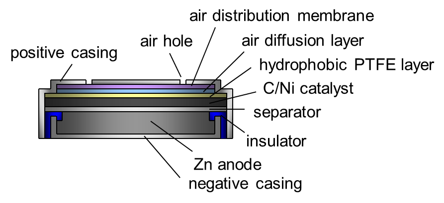
9.3. Secondary batteries
Like primary battery chemistries, a number of different secondary batteries are available, and new chemistries are frequently introduced in scientific journals. Moreover, the chemistries are similar to those in primary batteries but the secondary batteries have been designed for re-charging. They are therefore more complex in structure and typically have lower specific energies and energy densities than corresponding primary battery chemistries.
For secondary batteries, the nomenclature of the electrodes differs from the conventionally used anode and cathode. Instead of these terms, the negative and the positive electrode are used. This originates from the fact that during discharging the electrode at the lower potential functions is an anode but while charging it is a cathode. The situation is naturally opposite for the electrode with higher operation potential.
9.3.1 Lead acid battery
The first commercially available battery, the lead acid battery, was invented in the mid-1850, but significant technology improvements have been made since those days. This device is an economical choice for applications where weight is not critical. The affordable price results from low-priced and easily available raw materials and relatively simple fabrication methods. These batteries serve as uninterrupted power systems (UPS) to prevent critical power failure in stationary applications, for example in mobile phone repeater towers, internet hubs and hospitals. Despite their moderate energy density, lead acid batteries are also used as starter batteries in vehicles because they enable high power delivery during discharging, have a low self-discharge rate and are able to operate at low and even subzero temperatures.
Lead acid batteries designed for different application have similar chemistry but differ in technical implementation. For example, the design of the electrodes varies as well as the impregnation of cells with the electrolyte. In general, starting batteries requiring high power delivery, but no deep cycling, have thinner electrodes and are therefore lighter weight than batteries developed for deep cycling. The electrolyte is impregnated in X or gelled for mobile applications in particular.
As can be inferred from the name, lead is used in the both electrodes and concentrated sulfuric acid, approximately 37 vol% or 6-12 mol dm−3 as the electrolyte. Because of the slow water reaction kinetics on the lead-based electrodes, a high operation voltage (for an aqueous system) ranging from 2.15 V (fully charged) to 1.98 V (discharged battery) is obtained. During discharging, sulfuric acid is consumed and water formed, gradually diluting the electrolyte. This, in combination with the formation of lead sulfate, leads to an increase in the internal losses of the battery as the conductivity of both the electrodes and the electrolyte decrease and diffusion overpotentials increase.
The detailed reaction mechanism is very complex but it can be simplified with the following equations:
Negative electrode: Pb(s) + SO42-(aq) \(\ce{ <=> }\) PbSO4(s)
Pb(s) + H+(aq) + HSO4−(aq) \(\ce{ <=> }\) PbSO4(s) + 2H+(aq) + 2e−
Positive electrode: PbO2(s) + 4H+(aq) + SO42−(aq) + 2e− \(\ce{ <=> }\) PbSO4(s)+ 2H2O(l)
PbO2(s) + HSO4−(aq) + 3H+(aq) + 2e− \(\ce{ <=> }\) PbSO4(s) + 2H2O(l)
Net reaction: Pb + PbO2 + 2H2SO4 \(\ce{ <=> }\) 2PbSO4(s) + 2H2O(l)
Pb + PbO2 + 2H+ + 2HSO4− \(\ce{ <=> }\) 2PbSO4(s) + 2H2O(l)
In addition to these reactions, water electrolysis and the formation of H2 and O2 take place via side reactions.
9.3.2 Lithium ion battery
The lithium ion battery (LIB) has rapidly become the most popular battery in portable applications since it was introduced at the beginning of 1990s. These batteries have also been adopted as power sources in electric and hybrid vehicles and for peak power leveling in systems based on intermittent renewable energy. A high energy density combined with a relatively high power density has enabled them to achieve rapid success. LIBS have the downside that as they are rich in energy and contain a flammable electrolyte (LiF6P in a mixture of organic carbonates), large amounts of energy can be release if they are misused or in the case of a factory defect. In order to minimize the risk of of dangerous thermal runaway, each LIB is equipped with an electronic battery management system (BMS) that monitors its state and controls its charging.
Unlike other batteries, LIBs cover several different chemistries giving different characteristics to the batteries. In the first batteries, layered LiCoO2 was used for positive electrodes, and this material is still used in some devices for portable applications. For larger batteries LiCoO2 has been replaced with less expensive mixed oxides such as LiNixMnyCo(1-x-y)O2 and LiNixAlyCo(1-x-y)O2 with rather similar characteristics to LiCoO2. Yet another compound, LiFePO4 is considered a safe alternative with a longer cycle life. However, this chemistry makes a battery that has a lower energy density due to its lower operating voltage and a relatively low lithium ion storage capacity.
Since the first commercial LIBs, graphite has been the most popular negative electrode material. Li4Ti5O12 has been introduced as an alternative for applications that require a long cycle life and high charging rates but can accept the lower intrinsic energy density.
A scheme of the LIB operation is given in Figure 9.5. All the electrode materials set out above are based on the reversible intercalation reaction of the lithium ion in the lattice of the electrode material. It is concomitant with the change of the oxidation state of either of lithium (in graphite) or the transition metal in the host compound. For example, for the C|LiCoO2 chemistry these reactions are as follows:
Negative electrode: C6 + x Li+ + x e− \(\ce{ <=> }\) LixC6, x ≤ 1 Eo = 0.05-0.25 V vs. Li|Li+
Positive electrode: LiCoO2 \(\ce{ <=> }\) Li1-x CoO2 + x Li+ + x e− Eo = 3.0-4.5 V vs. Li|Li+
Net reaction: LiCoO2 + C6 \(\ce{ <=> }\) LixC + Li1−x CoO2

Figure 9.5. Operation principle of a LIB with LiCoO2 and C electrodes.
In commercial batteries, organic solvent-based electrolytes are used where LiPF6 serves as the charge carrier. The mixture typically consists of organic carbonates such as dimethyl carbonate, diethyl carbonate and ethyl methyl carbonate. The use of an organic electrolyte that has a higher electrochemical window than water enables the high voltage of the LIB, and the high energy density.
9.4. Fuel cells and flow batteries
Fuel cells enable environmentally friendly energy conversion of chemical energy into electricity with high efficiency of up to 83%. Although fuel cells are technologically viable, their high price hinders their adoption for a wider use. In addition to their mass manufacturing, materials development is a key problem to overcome.
Traditionally, fuel cells have been classified into different categories based on the electrolyte. Here, we introduce the polymer electrolyte fuel cell (PEFC) operating at low temperatures, and the high-temperature device, solid oxide fuel cell (SOFC). In the both devices, atmospheric air is often the oxidant. PEFCs mainly use hydrogen as the fuel although different alcohols and other small organic molecules have also been considered. Because of the higher operating temperature, an SOFC can also use synthetic gas, natural gas or biogas.
9.4.1 Polymer electrolyte fuel cell
Polymer electrolyte (membrane) fuel cells (PE(M)FC) have good energy density and can operate at a relatively low temperature range. They therefore provide an option for mobile applications such as electric vehicles and mobile phone chargers. However, they can be scaled up to serve as (local) stationary energy conversion units producing both heat and power, so they are also used for back-up power and auxiliary power unit applications.
The name PEMFC originates from the cation exchange membrane which serves as the solid electrolyte. The most commonly used membrane is Nafion®, a highly acidic material consisting of a perfluorinated polymer backbone with flexible sidechains containing ether linkages and terminal sulfite groups. Protons in these groups must be hydrated in order for the material to transfer protons (from the anode to the cathode). Consequently, operation is limited to the temperature range of liquid water.
Two half-reactions, hydrogen oxidation (HOR) and oxygen reduction (ORR), take place in a fuel cell. Both of these reactions are electrocatalytic i.e. their rates and mechanisms depend significantly on the electrode materials selected. Because of the acidic environment and relatively low operation temperatures, noble metal catalysts are needed to achieve reasonable reaction rates. The following reactions take place in acidic media:
anode: H2 \(\ce{ -> }\) 2 H+ + 2e− Eo = 0.00 vs. SHE
cathode: O2 + 4 H+ + 4 e− \(\ce{ -> }\) 2 H2O Eo = 1.23 vs. SHE
Net reaction: O2 + 2 H2 \(\ce{ -> }\) 2 H2O
Due to the high price of these catalysts, alternative catalyst materials and alkaline membrane-based technologies are under development.
9.4.2 Solid oxide fuel cell
Solid oxide fuel cells (SOFC) operate at high temperatures of 500-1,000oC to enhance conductivity of the ceramic electrolyte which is often yttria-stabilized zirconia (YSZ). Because of the high operation temperature and flexibility in the selection of the fuel, SOCFs are an appropriate choice for continuously operating stationary energy conversion systems. Moreover, the high operation temperature enhances electrochemical reactions, and no noble metal catalyst is needed to achieve appropriate reaction rates. Materials such as CoZrO2 or NiZrO2 cermet can serve as an anode while the Sr-doped LaMnO3 cathode is often used. In addition to appropriate functional properties, attention must be paid to matching thermal expansion coefficients when selecting the materials.
Using hydrogen as a fuel following reactions take place:
anode: H2 + O− \(\ce{ -> }\) H2O + e− Eo = 0.00 vs. SHE
cathode: O2 + 2 e− \(\ce{ -> }\) 2 O- Eo = 0.00 vs. SHE
net reaction: O2 + 2 H2 \(\ce{ -> }\) 2 H2O
9.4.3 Vanadium flow battery
A flow battery is kind of an intermediate between a battery and a fuel cell. In flow batteries, redox reactions take place in the reactor-type fuel cell but reactants are fed to the electrodes from external containers. A total of four containers is needed as depicted in Figure 9.6. Two of them contain reduced and oxide forms of the electrolyte fed to positive electrodes while the other pair enclose the respective electrolytes for the negative electrolyte. The flow direction is opposite during charging and discharging. The capacity of the system can therefore be adjusted by changing the size of the containers.
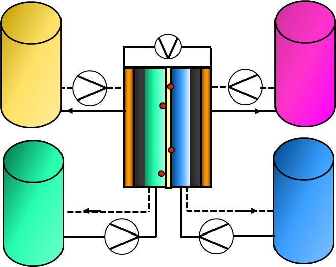
Figure 9.6. Construction of a flow battery.
Like in ordinary batteries, potential chemistries suitable for redox flow batteries are, in principle, unlimited. Vanadium flow batteries (VFB) are the only commercially available flow battery; their reactions are given here as an example. The forward direction corresponds to discharging and the backward direction to charging of the VFB.
negative electrode: V3+ + e− \(\ce{ <=> }\) V2+ Eo = -0.26 vs. SHE
positive electrode: VO2+ + H2O \(\ce{ <=> }\) VO2+ + 2 H+ + e− Eo = 1.00 vs. SHE
net reaction: V3+ + VO2+ + H2O \(\ce{ <=> }\) V2+ + VO2+ + 2 H+
Because of their bulky size, flow batteries are suitable for stationary energy storage applications. The electrodes must be made of conductive material enabling the reactions to occur, while a semi-permeable membrane enabling ion transport from one electrode to the other separates the catholyte and anolyte. For example, the in case of VFB discharge, protons are transported from the positive electrode to the negative one. Crossing of the vanadium species between catholyte and anolyte should, however, be avoided. Developmental challenges are related to the electrolyte price and abundancy, as well as to overall system costs. In addition to the VFB, zinc-bromine and sodium-sulfur flow batteries have also been studied, but they have suffered from stability problems.
9.5. Electrolyzers
The term “electrolyzer” refers to an electrochemical device in which decomposition of water into its molecular constituents, hydrogen and oxygen, takes place. The reactions are essentially the same as those occurring in a hydrogen fuel cell, but proceed in a reversed, non-spontaneous direction. Consequently, in an electrolyzer, electrical energy is converted into chemical bond energy. In this section, we introduce the two most common elecrolyzer systems, namely alkaline and polymer electrolyte electrolyzers.
Aqueous KOH electrolyte (see Figure 9.7)-based alkaline electrolyzer technology is more mature than acidic polymer electrolyte membrane electrolyzers (PEME). In the former system, a diaphragm is used to separate the anode and cathode compartments to prevent mixing of the generated H2 and O2 gases. The alkaline environment enables use of affordable electrode materials, and nickel-based (hydro)oxides are often used to catalyze the electrochemical reactions which proceed according to reactions:
Anode: 2 OH− \(\ce{ -> }\) ½ O2 + H2O + 2e− Eo = 0.00 vs. SHE
Cathode: 2H2O + 2e− \(\ce{ -> }\) H2 + OH− Eo = 0.00 vs. SHE
Overall: H2O \(\ce{ -> }\) H2 + ½ O2
PEME consists of similar components to PEFC: an acidic membrane electrolyte and noble metal electrodes. The benefits of a PEME over an alkaline electrolyzer are a higher current density and a shorter response time. PEMEs can also operate at higher pressures, and gas crossover is lower, producing high quality pure hydrogen. However, expensive noble metal-based catalysts, Pt for the cathode and Ir for the anode, are required and, hence, investment costs are high. Both the catalyst materials are scarce and alternatives are being sought. As stated above, reactions are similar to those in a PEFC but proceed in a reverse direction.
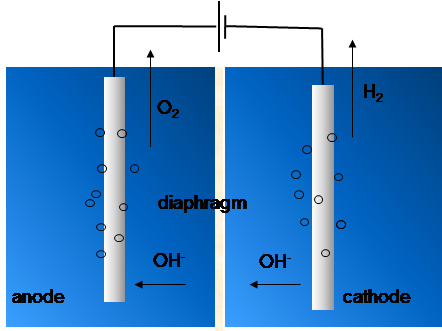
Figure 9.7. Operation principle of an alkaline electrolyzer for generating O2 and H2 from water.
Electrolyzers and other electrochemical devices enabling the conversion of electrical energy to chemical energy are attractive choices for renewable energy storage. In particular, the number of solar and wind power stations is drastically increasing, generating an excess of electricity during peak production hours. In order to maximize their benefit, this surplus needs to be converted or stored. Hydrogen has several uses: In addition to the above-mentioned fuel application, hydrogen is consumed in several chemical industry processes, and it can be mixed with natural or city gas or stored in containers for subsequent use.
10. List of symbols
A area; parameter in the Debye-Hückel theory; constant in Eq. (7.61)
a activity; ionic radius; Tafel slope
a± mean activity of the electrolyte
B parameter in the Debye-Hückel theory
b Tafel slope
C capacitance; dimensionless concentration c/c0
Cd capacitance of the diffuse layer
Cdl double layer capacitance
Cp pseudo capacitance
C2 capacitance of the inner layer
c molar concentration
c0 initial concentration
cb bulk concentration (typically equal to c0)
D diffusion coefficient; dissipation coefficient
D± diffusion coefficient of the electrolyte
d width of the channel (Fig 7.14)
E energy; cell potential; strength of the leectric field (chapter 3.1)
E0 standard potential
E0’ conditional potential (formal potential)
E1/2 half wave potential
Eeq equilibrium potential of the electrode
Ei initial potential of the linear potential sweep
Es switching potential of the linear potential sweep
Ediss dissipated energy
Estored stored energy
Ef Fermi energy
e elementary charge, 1.602×10⁻¹⁹ C
e− electron
F Faraday constant, 96485 C mol−1
f F/RT; activity coefficient on the mole fraction scale; friction coefficient; frequency
f0 charachteristic frequency of the quartz crystal
G Gibbs free energy
\( \Delta G_a^{\ddagger} \) activation energy of a reaction
H enthalpy
H(s) transfer function
H0 Hammet acidity function
H− Hammet basicity function
h thickness of a membrane; 2h = height of the channel (kuva 7.14)
I electric current; ionic strength
IC capacitive current
If Faradic current
Ilim electric current limited by diffusion
i current density
i0 exchange current density
id current density in the Cottrell experiment
ikin current density determined by kinetics
ilim current density limited by diffusion
J flux of the amount of substance (mol cm−2 s−1)
j imaginary unit, \( \sqrt{-1} \)
K equilibrium constant of a reaction
Ka association constant
Kb boiling point elevation constant
Kd dissociation constant
Kf freezing point depression constant li.e. cryoscopic constant
Kw ionic product of water, 10−14 M2 at 25 °C
k reaction rate constant; Bolzmann constant
k0 standard rate constant of an electrochemical reaction
kB Boltzmann constant 1,38×10⁻²³ J K−1
ka adsorption constant
kd desorption constant
kox rate constant of the oxidation reaction
kred rate constant of the reduction reaction
L inductance
l dimension of the electrode (Fig. (7.14))
M molar mass
m mass; molality
N number of particles
NA Avogadro constant, 6.023×10²³ mol−1
n amount of substance
O(s) output function
P pressure; probability
p partial pressure
Q electric charge
q amount of heat; charge density; parameter in the Bjerrum theory
qe electric charge in solution
q’ (adsorbed) charge of the inner layer
qd charge of the diffuse layer
R resistance; gas constant 8.314 J K−1 mol−1
Rct charge transfer resistance
Rp pseudo resistance
r rreaction rate; distance in spherical coordinates, radius
S entropy; function of linear potential sweep in Eq. (7.23)
s Laplace variable
T thermodynamic
(absolute) temperature; dimensionless time
t time; Hittorff transport number
ts time of the switching potential
U internal energy
U(s) input function
u mobility; dummy variable in integrals
V volume; potential field created by a single ion
\( \dot{V} \) rate of volume flow
\( \overline{V} \) partial molar volume
W work/energy
w work per particle
v rate of linear flow; reaction rate; rate of potentila sweep
x molar fraction; reaction coordinate
Y admittance
y activity coefficient on molality scale
Z impedance
z charge number; dimensionless location variable
\( \alpha \) degree of dissociation; charge transfer coefficient
\( \beta \) charge transfer coefficient
\( \Gamma \) surface concentration; gamma function
\( \Gamma \)i (1) relative surface concentration of species i
\( \gamma \) surface tension
\( \gamma \)i activity coefficient of an ion on molality scale
\( \gamma \)± mean activity coefficient on molality scale
\( \delta \) thickness of diffusion layer; integration step; phase difference between ac signals
\( \varepsilon \)0 relative permittivity of space 8.854×10⁻¹² F m−1
\( \varepsilon \)r relative permittivity
\( \eta \) overpotential E − Eeq; viscosity
\( \eta \)a activation overpotential
\( \eta \)c concentration overpotential
\( \theta \) exp[(nF)/(RT)(E
− E0’)]; surface coverage of hydrogen or oxygen
\( \theta \)i exp[(nF)/(RT)(Ei − E0’)]
\( \kappa \) conductivity of solution
\( \kappa \)−1 Debye length
\( \Lambda \) molar conductivity of solution
\( \lambda \)i molar conductivity of an ion
\( \lambda \) solvent reorganization energy in the Marcus theory
\( \mu \) chemical potential
\( \mu \)0 standard chemical potential
\( \tilde\mu \) electrochemical potential
\( \tilde\mu^0 \) standard electrochemical potential
\( \nu \) dynamic viscosity of solution
\( \pi \) osmotic pressure
\( \xi \) ratio of diffusion coefficients \( \sqrt{D_{\text{O}}/D_{\text{R}}} \)
\( \rho \) density of solution; charge density
\( \sigma \) constant of Warburg impedance; dimensionless sweep rate (nF)/(RT)×v
\( \sigma \)m surface charge of the electrode
\( \tau \) time constant of RC circuit t = RC, dimensionless time \( \tau=\sigma t \), transition time (7.50)
\( \Phi \) work funktion; osmotic coefficient
\( \phi \) galvani potential
\( \phi \)0 galvani potential of the solution at the surface of the electrode
\( \phi \)2 galvani potential at the interface of Helmholtz layer
\( \Delta_o^w\phi^0 \) standard potential of ion transfer from organic phase to water
\( \varphi \) dimensionless galvani potential (F\( \phi \))/(RT); surface coverage in Chapter 9
\( \psi \) outer potential; parameter in linear potential sweep, Eq (7.23)
\( \ \chi \) surface potential; dimensionless current
\( \omega \) angular frequency
11. Appendices
...11.1. Mean activity coefficients of electrolytes in water at 25 °C
|
Cl- |
|
|
|
|
|
|
|
Br- |
|
|
|
m |
HCl |
LiCl |
NaCl |
KCl |
MgCl2 |
CaCl2 |
|
m |
HBr |
LiBr |
|
0.1 |
0.796 |
0.790 |
0.778 |
0.770 |
0.528 |
0.518 |
|
0.1 |
0.805 |
0.796 |
|
0.2 |
0.767 |
0.757 |
0.735 |
0.718 |
0.488 |
0.472 |
|
0.2 |
0.782 |
0.766 |
|
0.3 |
0.756 |
0.744 |
0.710 |
0.688 |
0.476 |
0.455 |
|
0.3 |
0.777 |
0.756 |
|
0.4 |
0.755 |
0.740 |
0.693 |
0.666 |
0.474 |
0.448 |
|
0.4 |
0.781 |
0.752 |
|
0.5 |
0.757 |
0.739 |
0.681 |
0.649 |
0.480 |
0.448 |
|
0.5 |
0.789 |
0.753 |
|
0.6 |
0.763 |
0.743 |
0.673 |
0.637 |
0.490 |
0.453 |
|
0.6 |
0.801 |
0.758 |
|
0.7 |
0.772 |
0.748 |
0.667 |
0.626 |
0.505 |
0.460 |
|
0.7 |
0.815 |
0.767 |
|
0.8 |
0.783 |
0.755 |
0.662 |
0.618 |
0.521 |
0.470 |
|
0.8 |
0.832 |
0.777 |
|
0.9 |
0.795 |
0.764 |
0.659 |
0.610 |
0.543 |
0.484 |
|
0.9 |
0.850 |
0.789 |
|
1.0 |
0.809 |
0.774 |
0.657 |
0.604 |
0.569 |
0.500 |
|
1.0 |
0.871 |
0.803 |
|
1.2 |
0.84 |
0.796 |
0.654 |
0.593 |
0.630 |
0.539 |
|
1.2 |
0.917 |
0.837 |
|
1.4 |
0.876 |
0.823 |
0.655 |
0.586 |
0.708 |
0.587 |
|
1.4 |
0.969 |
0.874 |
|
1.6 |
0.916 |
0.853 |
0.657 |
0.580 |
0.802 |
0.644 |
|
1.6 |
1.029 |
0.917 |
|
1.8 |
0.96 |
0.885 |
0.662 |
0.576 |
0.914 |
0.712 |
|
1.8 |
1.094 |
0.964 |
|
2.0 |
1.009 |
0.921 |
0.668 |
0.573 |
1.051 |
0.792 |
|
2.0 |
1.168 |
1.015 |
|
2.5 |
1.147 |
1.026 |
0.668 |
0.569 |
1.538 |
1.063 |
|
2.5 |
1.389 |
1.161 |
|
3.0 |
1.316 |
1.156 |
0.714 |
0.569 |
2.320 |
1.483 |
|
3.0 |
1.674 |
1.341 |
|
3.5 |
1.518 |
1.317 |
0.746 |
0.572 |
3.550 |
2.080 |
|
3.5 |
|
1.584 |
|
4.0 |
1.762 |
0.510 |
0.783 |
0.577 |
5.530 |
2.930 |
|
4.0 |
|
1.897 |
|
4.5 |
2.04 |
1.741 |
0.826 |
0.583 |
8.720 |
4.170 |
|
4.5 |
|
2.28 |
|
5.0 |
2.38 |
2.020 |
0.874 |
|
13.920 |
5.890 |
|
5.0 |
|
2.74 |
|
5.5 |
2.77 |
2.340 |
0.928 |
|
|
8.180 |
|
5.5 |
|
3.27 |
|
6.0 |
3.22 |
2.720 |
0.986 |
|
|
11.110 |
|
6.0 |
|
3.92 |
|
NO3- |
|
|
|
|
|
|
|
ClO4- |
|
|
|
|
|
|
m |
HNO3 |
LiNO3 |
NaNO3 |
KNO3 |
Mg(NO3)2 |
Ca(NO3)2 |
m |
HClO4 |
LiClO4 |
NaClO4 |
Mg(ClO4)2 |
Ca(ClO4)2 |
|
|
0.1 |
0.791 |
0.788 |
0.762 |
0.739 |
0.522 |
0.488 |
|
0.1 |
0.803 |
0.812 |
0.775 |
0.577 |
0.557 |
|
0.2 |
0.754 |
0.752 |
0.703 |
0.663 |
0.480 |
0.429 |
|
0.2 |
0.778 |
0.794 |
0.729 |
0.565 |
0.532 |
|
0.3 |
0.735 |
0.736 |
0.666 |
0.614 |
0.467 |
0.397 |
|
0.3 |
0.768 |
0.792 |
0.701 |
0.576 |
0.532 |
|
0.4 |
0.725 |
0.728 |
0.638 |
0.576 |
0.465 |
0.378 |
|
0.4 |
0.766 |
0.798 |
0.683 |
0.599 |
0.544 |
|
0.5 |
0.720 |
0.726 |
0.617 |
0.545 |
0.469 |
0.365 |
|
0.5 |
0.769 |
0.808 |
0.668 |
0.633 |
0.564 |
|
0.6 |
0.717 |
0.727 |
0.599 |
0.519 |
0.478 |
0.356 |
|
0.6 |
0.776 |
0.820 |
0.656 |
0.673 |
0.589 |
|
0.7 |
0.717 |
0.729 |
0.583 |
0.496 |
0.488 |
0.349 |
|
0.7 |
0.785 |
0.834 |
0.648 |
0.723 |
0.618 |
|
0.8 |
0.718 |
0.733 |
0.570 |
0.476 |
0.501 |
0.344 |
|
0.8 |
0.795 |
0.852 |
0.641 |
0.780 |
0.654 |
|
0.9 |
0.721 |
0.737 |
0.558 |
0.459 |
0.518 |
0.340 |
|
0.9 |
0.808 |
0.869 |
0.635 |
0.849 |
0.695 |
|
1.0 |
0.724 |
0.743 |
0.548 |
0.443 |
0.536 |
0.338 |
|
1.0 |
0.823 |
0.887 |
0.629 |
0.925 |
0.743 |
|
1.2 |
0.734 |
0.757 |
0.530 |
0.414 |
0.580 |
0.337 |
|
1.2 |
0.858 |
0.931 |
0.622 |
1.112 |
0.853 |
|
1.4 |
0.745 |
0.774 |
0.514 |
0.390 |
0.631 |
0.337 |
|
1.4 |
0.900 |
0.979 |
0.616 |
1.355 |
0.992 |
|
1.6 |
0.758 |
0.792 |
0.501 |
0.369 |
0.691 |
0.339 |
|
1.6 |
0.947 |
1.034 |
0.613 |
1.667 |
1.161 |
|
1.8 |
0.775 |
0.812 |
0.489 |
0.350 |
0.758 |
0.342 |
|
1.8 |
0.998 |
1.093 |
0.611 |
2.08 |
1.372 |
|
2.0 |
0.793 |
0.835 |
0.478 |
0.333 |
0.835 |
0.347 |
|
2.0 |
1.055 |
1.158 |
0.609 |
2.59 |
1.634 |
|
2.5 |
0.846 |
0.896 |
0.455 |
0.297 |
1.088 |
0.362 |
|
2.5 |
1.227 |
1.350 |
0.609 |
4.78 |
2.62 |
|
3.0 |
0.909 |
0.966 |
0.437 |
0.269 |
1.449 |
0.382 |
|
3.0 |
1.448 |
1.582 |
0.611 |
8.99 |
4.21 |
|
3.5 |
|
1.044 |
0.422 |
0.246 |
1.936 |
0.407 |
|
3.5 |
1.726 |
1.866 |
0.617 |
17.26 |
6.76 |
|
4.0 |
|
1.125 |
0.408 |
|
2.59 |
0.438 |
|
4.0 |
2.08 |
2.18 |
0.626 |
33.3 |
10.77 |
|
4.5 |
|
1.215 |
0.396 |
|
3.50 |
0.472 |
|
4.5 |
2.53 |
|
0.637 |
|
17.02 |
|
5.0 |
|
1.310 |
0.386 |
|
4.74 |
0.510 |
|
5.0 |
3.11 |
|
0.649 |
|
26.7 |
|
5.5 |
|
1.407 |
0.378 |
|
|
0.551 |
|
5.5 |
3.83 |
|
0.662 |
|
41.7 |
|
6.0 |
|
1.506 |
0.371 |
|
|
0.596 |
|
6.0 |
4.76 |
|
0.677 |
|
63.7 |
|
OH- |
|
|
|
|
SO4- |
|
|
|
|
m |
LiOH |
NaOH |
KOH |
|
m |
Li2SO4 |
Na2SO4 |
K2SO4 |
|
0.1 |
0.718 |
0.764 |
0.776 |
|
0.1 |
0.478 |
0.452 |
0.436 |
|
0.2 |
0.663 |
0.725 |
0.739 |
|
0.2 |
0.406 |
0.371 |
0.356 |
|
0.3 |
0.628 |
0.706 |
0.721 |
|
0.3 |
0.369 |
0.325 |
0.313 |
|
0.4 |
0.603 |
0.695 |
0.713 |
|
0.4 |
0.344 |
0.294 |
0.283 |
|
0.5 |
0.583 |
0.688 |
0.712 |
|
0.5 |
0.326 |
0.270 |
0.261 |
|
0.6 |
0.566 |
0.683 |
0.712 |
|
0.6 |
0.313 |
0.252 |
0.243 |
|
0.7 |
0.553 |
0.680 |
0.715 |
|
0.7 |
0.303 |
0.237 |
0.229 |
|
0.8 |
0.541 |
0.677 |
0.721 |
|
0.8 |
0.295 |
0.225 |
|
|
0.9 |
0.532 |
0.676 |
0.728 |
|
0.9 |
0.288 |
0.213 |
|
|
1.0 |
0.523 |
0.677 |
0.735 |
|
1.0 |
0.283 |
0.204 |
|
|
1.2 |
0.512 |
0.679 |
0.754 |
|
1.2 |
0.277 |
0.1890 |
|
|
1.4 |
0.503 |
0.684 |
0.778 |
|
1.4 |
0.273 |
0.1774 |
|
|
1.6 |
0.496 |
0.690 |
0.804 |
|
1.6 |
0.271 |
0.1680 |
|
|
1.8 |
0.489 |
0.698 |
0.832 |
|
1.8 |
0.270 |
0.1605 |
|
|
2.0 |
0.485 |
0.707 |
0.863 |
|
2.0 |
0.269 |
0.1544 |
|
|
2.5 |
0.475 |
0.741 |
0.947 |
|
2.5 |
0.280 |
0.1441 |
|
|
3.0 |
0.467 |
0.782 |
1.051 |
|
3.0 |
0.294 |
0.1387 |
|
|
3.5 |
0.460 |
0.833 |
1.181 |
|
3.5 |
|
0.1367 |
|
|
4.0 |
0.454 |
0.901 |
1.314 |
|
4.0 |
|
0.1376 |
|
|
4.5 |
|
0.982 |
1.49 |
|
|
|
|
|
|
5.0 |
|
1.074 |
1.67 |
|
|
|
|
|
|
5.5 |
|
1.178 |
1.90 |
|
|
|
|
|
|
6.0 |
|
1.296 |
2.14 |
|
|
|
|
|
11.2. Values of molar conductivity and diffusion coefficient at infinite dilution in water at 25 °C
For the molar conductivity \( \lambda_i \) and the equivalent conductivity \( \lambda_{\text{eq}, i} \), the following equation holds: \( \lambda_i=|z_i| \cdot\lambda_{\text{eq},i} \), where \( z_i \) is the charge of the ion. The tabulated values are molar conductivities at infinite dilution (\( \lambda_i^0 \)).
|
|
|
|
|
|
|
|
|
|
|
|
|
|
|
|||||||
|
|
ion |
zi |
λi0 |
Di \( \times \) 105 cm2/s-1 |
ion |
zi |
λi0 |
Di \( \times \) 105 cm2/s-1 |
|
|
|
H+ |
1 |
349.8 |
9.312 |
OH– |
-1 |
197.6 |
5.260 |
|
|
|
Li+ |
1 |
38.69 |
1.030 |
Cl– |
-1 |
76.34 |
2.032 |
|
|
|
Na+ |
1 |
50.11 |
1.334 |
Br– |
-1 |
78.3 |
2.084 |
|
|
|
K+ |
1 |
73.52 |
1.957 |
I– |
-1 |
76.8 |
2.044 |
|
|
|
NH4+ |
1 |
73.4 |
1.954 |
NO3– |
-1 |
71.44 |
1.902 |
|
|
|
Ag+ |
1 |
61.92 |
1.648 |
HCO3– |
-1 |
41.5 |
1.105 |
|
|
|
Tl+ |
1 |
74.7 |
1.989 |
HCO2– |
-1 |
54.6 |
1.454 |
|
|
|
Mg2+ |
2 |
106.12 |
0.7063 |
CH3CO2– |
-1 |
40.9 |
1.089 |
|
|
|
Ca2+ |
2 |
119.00 |
0.7920 |
SO42 – |
-2 |
160 |
1.065 |
|
|
|
Sr2+ |
2 |
118.92 |
0.7914 |
Fe(CN)63 – |
-3 |
303 |
0.896 |
|
|
|
Ba2+ |
2 |
127.28 |
0.8471 |
Fe(CN)64 – |
-4 |
444 |
0.739 |
|
|
|
Cu2+ |
2 |
108 |
0.72 |
IO4– |
-1 |
54.38 |
1.448 |
|
|
|
Zn2+ |
2 |
106 |
0.71 |
ClO4– |
-1 |
67.32 |
1.792 |
|
|
|
La3+ |
3 |
208.5 |
0.617 |
BrO3– |
-1 |
55.78 |
1.485 |
|
|
|
Co(NH3)63 + |
3 |
306.9 |
0.908 |
HSO4– |
-1 |
50 |
1.33 |
|
|
|
|
|
|
|
|
|
|
|
|
11.3. Relations of complex numbers
Complex number: \( z=x+iy \), where \( i=\sqrt{{-1}} \) is imaginary unit
Complex conjugate: \( z^*=x-iy \)
In polar coordinates: \( z=re^{i\varphi} \)
\( r=\sqrt{zz^*}=\sqrt{x^2+y^2} \)
\( \varphi=\text{atan}(y/x) \)
Euler's formula: \( re^{\pm i\varphi}=r(\cos\varphi\pm i\sin\varphi) \), where
\( x=r\cos(\varphi) \) and \( y=r\sin(\varphi) \)
De Moivre's formula: \( (\cos\varphi+i\sin\varphi)^n=\cos(n\varphi)+i\sin(n\varphi) \)
Relationship between triginimetric and hyberbolic functions:
\( \sin\varphi=\frac{1}{2i}(e^{i\varphi}-e^{-i\varphi})=-i\sinh(i\varphi) \) or \( \sin(i\varphi)=i\sinh(\varphi) \)
\( \cos\varphi=\frac{1}{2}(e^{i\varphi}-e^{-i\varphi})=\cosh(i\varphi) \) or \( \cos(i\varphi)=\cosh(\varphi) \)
\( \tan\varphi=\frac{1}{i}\frac{e^{i\varphi}-e^{-i\varphi}}{e^{i\varphi}+e^{-i\varphi}}=-i\tanh(i\varphi) \) or \( \tan(i\varphi)=i\tanh(\varphi) \)
\( \cot\varphi=\frac{1}{i}\frac{e^{i\varphi}+e^{-i\varphi}}{e^{i\varphi}-e^{-i\varphi}}=-i\coth(i\varphi) \) or \( \cot(i\varphi)=i\coth(\varphi) \)
Exponentials of the imaginary unit:
\( i=e^{i\pi/2} \Rightarrow i^n=(e^{i\pi/2})^n=e^{in\pi/2}=\cos(\frac{n\pi}{n})+i\sin(\frac{n\pi}{2}) \)
E.g. \( \sqrt{i}=i^{1/2}=\cos(\frac{\pi}{4})+i\sin(\frac{\pi}{4})=\frac{1+i}{\sqrt{2}} \)
Note that in this book, the imaginary unit i has been replaced by j because i is reserved for the symbol of electric current density.
11.4. Laplace transforms
| Definition: | \( \mathcal{L}\{f(t)\}=F(s)=\int_0^{\infty}{e^{-st}}f(t)dt \) |
||
|---|---|---|---|
| Derivation: | \( \mathcal{L}\{f'(t)\}=sF(s)-f(0) \) |
||
| Integration |
\( \mathcal{L}\left\{\int_{0}^{t}{f(u)du}\right\}=\frac{1}{s}F(s) \) \( \mathcal{L}\left\{ \int_{0}^{t}\int_{0}^{u}{f(v)dvdu} \right\}=\frac{1}{s^2}F(s) \) |
||
| Linearity: | \( \mathcal{L}\{Af(t)+Bg(t)\}=AF(s)+BG(s) \) |
||
| Transfer in Laplace domain: | \( \mathcal{L}\{e^{at}f(t)\}=F(s-a) \) |
||
| Transfer in time domain: | \( \mathcal{L}\{f(t-a)H_s(t-a)\}=e^{-as}F(s), a>0 \) \( H_s(t-a)=\begin{cases}0,t<\\1, t>a\end{cases} \) Heaviside step function |
||
| Convolution: | \( \mathcal{L}\left\{\int_{0}^{t}{f(t-u)g(u)du}\right\}=F(s)G(s) \) |
||
| Heaviside theory: | \( \mathcal{L}\left\{\sum\limits_{n=1}^m{\frac{p(a_n)}{q'(a_n)}e^{a_nt}}\right\}=\frac{P(s)}{Q(s)} \), where roots of Q(s) are: a1, a2, ..., an. |
Most common transforms in electrochemistry
f(t) |
F(s) |
||
|---|---|---|---|
| ---------------------------------------------------------------------------- | ------------------------- | ||
| \(1\) | \(\displaystyle \frac{1}{s} \) |
||
| \( t \) |
\(\displaystyle \frac{1}{s^2} \) |
||
| \(\displaystyle \frac{t^{n-1}}{(n-1)!} \) |
\(\displaystyle \frac{1}{s^n} \) | ||
| \(\displaystyle\frac{1}{\sqrt{\pi t}}\) |
\( \displaystyle\frac{1}{\sqrt{s}} \) |
||
| \(\displaystyle2\sqrt{\frac{t}{\pi}}\) |
\(\displaystyle \frac{1}{s\sqrt{s}} \) |
||
| \(\displaystyle e^{-at} \) |
\(\displaystyle \frac{1}{s+a} \) |
||
| \( \sin(\omega t) \) |
\(\displaystyle \frac{\omega}{s^2+\omega^2} \) |
||
| \( \cos(\omega t) \) |
\(\displaystyle \frac{s}{s^2+\omega^2} \) |
||
| \( \displaystyle\frac{1}{\sqrt{\pi t}}-ae^{a^2t}\text{erfc}(a\sqrt{t}) \) |
\(\displaystyle \frac{1}{\sqrt{s}+a} \) |
||
| \( \displaystyle\frac{1}{\sqrt{\pi t}}+ae^{a^2t}\text{erf}(a\sqrt{t}) \) |
\(\displaystyle \frac{\sqrt{s}}{s-a^2} \) |
||
| \( \displaystyle e^{a^2t}\text{erf}({a\sqrt{t}}) \) |
\(\displaystyle \frac{a}{\sqrt{s}(s-a^2)} \) |
||
| \( \displaystyle1-e^{a^2t}\text{erfc}({a\sqrt{t}}) \) |
\(\displaystyle \frac{a}{s(\sqrt{s}+a)} \) |
||
| \( \displaystyle e^{a^2t}\text{erfc}({a\sqrt{t}}) \) |
\(\displaystyle \frac{1}{\sqrt{s}(\sqrt{s}+a)} \) |
||
| \( \displaystyle\frac{a}{2\sqrt{\pi t^3}}\exp\left(-\frac{a^2}{4t}\right) \) |
\(\displaystyle e^{-a\sqrt{s}},a \geq0 \) |
||
\(\displaystyle \frac{1}{\sqrt{\pi t}} \text{exp}\left(-\frac{a^2}{4t}\right) \) |
\(\displaystyle \frac{1}{\sqrt{s}}e^{-a\sqrt{s}}, a \geq0 \) | ||
| \( \displaystyle\text{erfc}\left(\frac{a}{2\sqrt{t}}\right) \) |
\(\displaystyle \frac{1}{s}e^{-a\sqrt{s}}, a \geq0 \) |
||
| \(\displaystyle 2\sqrt{\frac{t}{\pi}}\exp\left(-\frac{a^2}{4t}\right)-a\text{ erfc}\left(\frac{a}{2\sqrt{t}}\right) \) |
\(\displaystyle \frac{1}{s\sqrt{s}}e^{-a\sqrt{s}}, a \geq0 \) |
||
| \(\displaystyle \frac{1}{\sqrt{\pi t}}\exp\left(-\frac{a^2}{4t}\right)-be^{ab+b^2t}\text{erfc}\left(\frac{a}{2\sqrt{t}}+b\sqrt{t}\right) \) |
\(\displaystyle \frac{e^{-a\sqrt{s}}}{\sqrt{s}+b}, a \geq0 \) |
11.5. Standard reduction potentials in water at 25 °C
Based on the international convention that E0(H+/H2) \( \equiv \) 0 V at all temperatures.
Electrode E0/V Reaction
__________________________________________________________________________
Li+|Li -3.040 Li+ + e- → Li
K+|K -2.924 K+ + e- → K
Rb+|Rb -2.924 Rb+ + e- → Rb
Na+|Na -2.713 Na+ + e- → Na
Mg2+|Mg -2.356 1/2 Mg2+ + e- → 1/2 Mg
Al3+|Al -1.676 1/3 Al3+ + e- → 1/3 Al
OH-|H2|Pt -0.828 H2O + e- → 1/2 H2 + OH-
Zn2+|Zn -0.7626 1/2 Zn2+ + e- → 1/2 Zn
S2-|Ag2S(s)|Ag -0.691 1/2 Ag2S + e- → Ag + 1/2 S2-
Br-|TlBr(s)|Tl -0.658 TlBr + e-→ Tl + Br-
Fe2+|Fe -0.44 1/2 Fe2+ + e- → 1/2 Fe
Cr3+, Cr2+|Pt -0.424 Cr3+ + e- → Cr2+
Cd2+|Cd -0.403 1/2 Cd2+ + e- → 1/2 Cd
I-|PbI2(s)|Pb -0.365 1/2 PbI2 + e- → 1/2 Pb + I-
SO42 -|PbSO4(s)|Pb -0.359 1/2 PbSO4 + e- → 1/2 Pb + 1/2 SO42 -
F-|PbF2(s)|Pb -0.344 1/2 PbF2 + e- → 1/2 Pb + F-
Tl+|Tl -0.3363 Tl+ + e- → Tl
Br-|PbBr2(s)|Pb -0.280 1/2 PbBr2 + e- → 1/2 Pb + Br
Co2+|Co -0.277 1/2 Co2+ + e- → 1/2 Co
Cl-|PbCl2(s)|Pb -0.268 1/2 PbCl2 + e- → 1/2 Pb + Cl-
Ni2+|Ni -0.257 1/2 Ni2+ + e- → 1/2 Ni
I-|AgI(s)|Ag -0.1522 AgI + e- → Ag + I-
Sn2+|Sn -0.136 1/2 Sn2+ + e- → 1/2 Sn
Pb2+|Pb -0.1251 1/2 Pb2+ + e- → 1/2 Pb
|
TiO2+. Ti3+|Pt 0.10 TiO2+ + 2H+ + e- → Ti3++ H2O
Br-|AgBr(s)|Ag 0.0711 AgBr + e- → Ag + Br-
Sn4+, Sn2+|Pt 0.15 1/2 Sn4+ + e- → 1/2 Sn2+
Cu2+, Cu+|Pt 0.159 Cu2+ + e- → Cu+
Cl-|AgCl(s)|Ag 0.2223 AgCl + e- → Ag + Cl-
Cl-|Hg2Cl2(s)|Hg 0.2682* 1/2Hg2Cl2 + e- → Hg + Cl-
Cu2+|Cu 0.340 1/2 Cu2+ + e- → 1/2 Cu
OH-|O2|Pt 0.401 1/2 O2 + H2O + 2e- → 2 OH-
CO32 -|Ag2CO3(s)|Ag 0.47 1/2 Ag2CO3 + e- → Ag + 1/2 CO32 -
Cu+|Cu 0.520 Cu+ + e- → Cu
I-|I2(s)|Pt 0.5355 1/2 I2 + e- → I-
SO42 -|Hg2SO4(s)|Hg 0.613 1/2 Hg2SO4 + e- → Hg + 1/2 SO42 -
SO42 -|Ag2SO4(s)|Ag 0.654 1/2 Ag2SO4 + e- → Ag + 1/2 SO42 -
H+|quinhydrone(s)|Pt 0.6996 1/2 C6H4O2 + H+ + e- → 1/2 C6H6O2
Fe3+, Fe2+|Pt 0.771 Fe3+ + e- → Fe2+
Hg22 +|Hg 0.796 1/2 Hg22 + + e- → Hg
Ag+|Ag 0.799 Ag+ + e- → Ag
Hg2+, Hg22 +|Pt 0.911 Hg2+ + e- → 1/2 Hg22 +
Br-|Br2(l)|Pt 1.065 1/2 Br2(l) + e- → Br-
H+|O2|Pt 1.229 1/2 O2 + 2 H+ + 2 e- → H2O
Tl3+, Tl+|Pt 1.25 1/2 Tl3+ + e- → 1/2 Tl+
Cl-|Cl2(g)|Pt 1.3583 1/2 Cl2(g) + e- → Cl-
Pb2+|PbO2|Pb 1.468 1/2 PbO2(s) + 2H++ e- → 1/2 Pb2+ + H2O
Au3+|Au 1.52 1/3 Au3+ + e- → 1/3 Au
SO42 -|PbO2(s)|PbSO4(s)|Pb 1.698 PbO2 + SO42 - + 4 H+ + 2 e- → PbSO4 + 2 H2O
Ce4+, Ce3+|Pt 1.72 Ce4+ + e- → Ce3+
Co3+, Co2+|Pt 1.92 Co3+ + e- → Co2+
F-|F2(g)|Pt 2.87 1/2 F2(g) + e- → F-
HF(aq)|F2(g)|Pt 3.053 H+ + 1/2 F2(g) + e- → HF(aq)