Differential and Integral Calculus
| Site: | MyCourses |
| Course: | MS-A0111 - Differential and Integral Calculus 1, Lecture, 13.9.2021-27.10.2021 |
| Book: | Differential and Integral Calculus |
| Printed by: | Guest user |
| Date: | Wednesday, 19 February 2025, 1:10 AM |
1. Sequences
Basics of sequences
This section contains the most important definitions about sequences. Through these definitions the general notion of sequences will be explained, but then restricted to real number sequences.
Definition: Sequence
Let  be a non-empty set. A sequence is a function:

Occasionally we speak about a sequence in .
Note. Characteristics of the set  give certain characteristics to the sequence. Because is ordered, the terms of the sequence are ordered.
Definition: Terms and Indices
A sequence can be denoted denoted as
 = (a_{n})_{n\in\mathbb{N}} = (a_{n})_{n=1}^{\infty} = (a_{n})_{n}")
instead of .") The numbers
The numbers  are called the terms of the sequence.
Because of the mapping
 we can assign a unique number
  to each term. We write this number as a subscript and define it as the index; it follows that we can identify any term of the sequence by its index.
| n | 1 | 2 | 3 | 4 | 5 | 6 | 7 | 8 | 9 |  |
|---|---|---|---|---|---|---|---|---|---|---|
 |
|
|
|
|
|
|
|
|
||
 |
 |
 |
 |
 |
 |
 |
 |
 |
 |
|
A few easy examples
Example 1: The sequence of natural numbers
The sequence _{n}") defined by
defined by  is called the sequence of natural numbers. Its first few terms are:
 This special sequence has the property that every term is the same as its index.
![]()
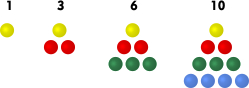
Example 2: The sequence of triangular numbers
Triangular numbers get their name due to the following geometric visualization: Stacking coins to form a triangular shape gives the following diagram:
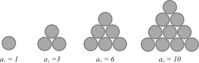
To the first coin in the first layer we add two coins in a second layer to form the second picture  . In turn, adding three coins to forms
  . From a mathematical point of view, this sequence is the result of summing natural numbers. To calculate the 10th triangular number we need to add the first 10 natural numbers:
 In general form the sequence is defined as:
 +n.")
This motivates the following definition:
Notation and Definition: Sum sequence
Let _n, a_n: \mathbb{N}\to M") be a sequence with terms
be a sequence with terms  , the sum is written:
 The sign
  is called sigma. Here, the index
  increases from 1 to
  .
.
Sum sequences are sequences whose terms are formed by summation of previous terms.
Thus the nth triangular number can be written as:

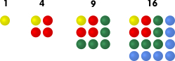
Example 3: Sequence of square numbers
The sequence of square numbers _n") is defined by:
is defined by:  . The terms of this sequence can also be illustrated by the addition of coins.
Interestingly, the sum of two consecutive triangular numbers is a square number. So, for example, we have:  and
and  . In general this gives the relationship:

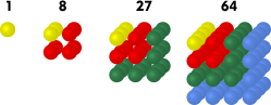
Example 4: Sequence of cube numbers
Analogously to the sequence of square number, we give the definition of cube numbers as  The first terms of the sequence are:
 ") .
.
Example 5.
Let with  be the sequence of square numbers
\end{aligned}") and define the function
and define the function  = 2n") . The composition
. The composition _n") yields:
yields:
_n &= (q_2,q_4,q_6,q_8,q_{10},\ldots) \\
&= (4,16,36,64,100,\ldots).\end{aligned}")
Definition: Sequence of differences
Given a sequence _{n}=a_{1},\, a_{2},\, a_{3},\ldots,\, a_{n},\ldots") ; then
; then
_{n}:=a_{2}-a_{1}, a_{3}-a_{2},\dots") is called the 1st difference sequence of
is called the 1st difference sequence of
The 1st difference sequence of the 1st difference sequence is called the 2nd difference sequence. Analogously the th difference< sequence is defined.
Example 6.
Given the sequence _n") with
with  , i.e.
_n &= (1,3,6,10,15,21,28,36,\ldots)\end{aligned}") Let
Let _n") be its 1st difference sequence. Then it follows that
be its 1st difference sequence. Then it follows that
_n &= (a_2-a_1, a_3-a_2, a_4-a_3,\ldots) \\
&= (2,3,4,5,6,7,8,9)\end{aligned}") A term of has the general form
A term of has the general form
^2+(n+1)}{2} - \frac{n^2+n)}{2} \\
&= \frac{(n+1)^2+(n+1)-n^2 - n }{2} \\
&= \frac{(n^2+2n+1)+1-n^2}{2} \\
&= \frac{2n+2}{2} \\
&= n + 1.\end{aligned}")
Some important sequences
There are a number of sequences that can be regarded as the basis of many ideas in mathematics, but also can be used in other areas (e.g. physics, biology, or financial calculations) to model real situations. We will consider three of these sequences: the arithmetic sequence, the geometric sequence, and Fibonacci sequence, i.e. the sequence of Fibonacci numbers.
The arithmetic sequence
There are many definitions of the arithmetic sequence:
Definition A: Arithmetic sequence
A sequence is called the arithmetic sequence, when the difference  between two consecutive terms is constant, thus:

Note: The explicit rule of formation follows directly from definition A:
\cdot d") For the th term of an arithmetic sequence we also have the recursive formation rule:
For the th term of an arithmetic sequence we also have the recursive formation rule:

Definition B: Arithmetic sequence
A non-constant sequence is called an arithmetic sequence (1st order) when its 1st difference sequence is a sequence of constant value.
This rule of formation gives the arithmetic sequence its name: The middle term of any three consecutive terms is the arithmetic mean of the other two, for example:

Example 1.
The sequence of natural numbers
_n = (1,2,3,4,5,6,7,8,9,\ldots)") is an arithmetic sequence, because the difference,
is an arithmetic sequence, because the difference,  , between two consecutive terms is always given as
  .
.
The geometric sequence
The geometric sequence has multiple definitions:
Definition: Geometric sequence
A sequence is called a geometric sequence when the ratio of any two consecutive terms is always constant  , thus

Note.The recursive relationship
 of the terms of the geometric sequence and the explicit formula for the calculation of the n
th term of a geometric sequence
of the terms of the geometric sequence and the explicit formula for the calculation of the n
th term of a geometric sequence
 follows directly from the definition.
Again the name and the rule of formation of this sequence are connected: Here, the middle term of three consecutive terms is the geometric mean of the other two, e.g.:

Example 2.
Let  and
and  be fixed positive numbers. The sequence with
  , i.e.
 = \left( a, aq, aq^2, aq^3,\ldots \right)") is a geometric sequence. If
is a geometric sequence. If  the sequence is monotonically increasing. If it is strictly decreasing. The corresponding range
  is finite in the case
  (namely, a singleton), otherwise it is infinite.
The Fibonacci sequence
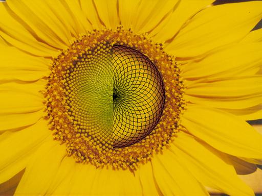
The Fibonacci sequence is famous because it plays a role in many biological processes, for instance in plant growth, and is frequently found in nature. The recursive definition is:
Definition: Fibonacci sequence
Let  and let
 for
for  . The sequence is then called the Fibonacci sequence. The terms of the sequence are called the Fibonacci numbers.
The sequence is named after the Italian mathematician Leonardo of Pisa (ca. 1200 AD), also known as Fibonacci (son of Bonacci). He considered the size of a rabbit population and discovered the number sequence:
,")
Example 3.
The structure of sunflower heads can be described by a system of two spirals, which radiate out symmetrically but contra rotating from the centre; there are 55 spirals which run clockwise and 34 which run counter-clockwise.
Pineapples behave very similarly. There we have 21 spirals running in one direction and 34 running in the other. Cauliflower, cacti, and fir cones are also constructed in this manner.
Convergence, divergence and limits
The following chapter deals with the convergence of sequences. We will first introduce the idea of zero sequences. After that we will define the concept of general convergence.
Preliminary remark: Absolute value in 
The absolute value function  is fundamental in the study of convergence of real number sequences. Therefore we should summarise again some of the main characteristics of the absolute value function:
Definition: Absolute Value
For any given number  its absolute value
  is defined by

Graph of the absolute value function
Theorem: Calculation Rule for the Absolute Value
For  the following is always true:

 if and only if
 (Multiplicativity)
 (Triangle Inequality)
Parts 1.-3. Results follow directly from the definition and by dividing it up into separate cases of the different signs of  and
and 
Part 4. Here we divide the triangle inequality into different cases.
Case 1.
First let  . Then it follows that
 and the desired inequality is shown.
Next let  . Then:
=(-x)+ (-y)=|x|+|y|\end{aligned}")
Finally we consider the case  and . Here we have two subcases:
For
 we have
  and thus
  from the definition of absolute value. Because then and therefore also
  . Overall we have:

For
 then
then  . We have
 =-x-y") . Because
. Because  , we have
  and thus
  . Overall we have:

The case and  we prove it analogously to the case 3, in which and are exchanged.

Zero sequences
Definition: Zero sequence
A sequence s called a zero sequence, if for every  there exists an index
  such that
 for every
  . In this case we also say that the sequence converges to zero.
Informally: We have a zero sequence, if the terms of the sequence with high enough indices are arbitrarily close to zero.
Example 1.
The sequence defined by  , i.e.
 :=\left(\frac{1}{1},\frac{1}{2},\frac{1}{3},\frac{1}{4},\ldots\right)") is called the harmonic sequence. Clearly, it is positive for all , however as increases the absolute value of each term decreases getting closer and closer to zero.
is called the harmonic sequence. Clearly, it is positive for all , however as increases the absolute value of each term decreases getting closer and closer to zero.
Take for example  , then choosing the index
  , it follows that , for all
  .
.
The harmonic sequence converges to zero
Example 2.
Consider the sequence
_n \text{ where } a_n:=\frac{1}{\sqrt{n}}.") Let
Let  .We then obtain the index
  in this manner that for all terms where
  .
.
Note. To check whether a sequence is a zero sequence, you must choose an (arbitrary)  where
where  . Then search for a index
  , after which all terms are smaller then said
  .
.
Example 3.
We consider the sequence , defined by
^n \cdot \frac{1}{n^2}.")
Because of the factors ^n") two consecutive terms have different signs; we call a sequence whose signs change in this way an alternating sequence.
two consecutive terms have different signs; we call a sequence whose signs change in this way an alternating sequence.
We want to show that this sequence is a zero sequence. According to the definition we have to show that for every there exist  , such that we have the inequality:
 for every term where .
Firstly we let be an arbitrary constant. Because the inequality  must hold true for an arbitrary we must find the index which depends on each . More exactly: The inequality
  must be true for the index . Solve for :
 this index gives our desired characteristic for every .
Negative examples
The following are examples of non-convergent alternating sequences:
^n")
^n \cdot n")
Theorem: Characteristics of Zero sequences
Let and be two sequences. Then:
Let
be a zero sequence, if  or
or  for all then is also a zero sequence.
Let
be a zero sequence, if  for all then is also a zero sequence.
Let
be a zero sequence, then _n") where
where  is also a zero sequence.
If
and are zero sequences, then _n") is also a zero sequence.
is also a zero sequence.
Parts 1 and 2. If is a zero sequence, then according to the definition there is an index , such that  for every and an arbitrary
  . But then we have
  ; this proves parts 1 and 2 are correct.
Part 3. If  , then the result is trivial. Let
  and choose such that
 for all .
Rearranging we get:
for all .
Rearranging we get:

Part 4.
Because is a zero sequence, by the definition we have for all . Analogously, for the zero sequence there is a  with
with  for all
  .
.
Then for all ") it follows (using the triangle inequality) that:
it follows (using the triangle inequality) that:

Convergence, divergence
The concept of zero sequences can be expanded to give us the convergence of general sequences:
Definition: Convergence and Divergence
A sequence is called convergent to  , if for every
  there exists a
  such that:

An equivalent definition can be defined by:
A sequence is called convergent to , if _{n}") is a zero sequence.
is a zero sequence.
Example 4.
We consider the sequence where
 By plugging in large values of , we can see that for
 and therefore we can postulate that the limit is
  .
.
For a vigorous proof, we show that for every there exists an index  , such that for every term with
  the following relationship holds:

Firstly we estimate the inequality:
}{n^2+1}\right| \\
=&\left|\frac{2n^2+1-2n^2-2}{n^2+1}\right| \\
=&\left|-\frac{1}{n^2+1}\right| \\
=&\left|\frac{1}{n^2+1}\right| \\")
Now, let be an arbitrary constant. We then choose the index , such that
 Finally from the above inequality we have:
 Thus we have proven the claim and so by definition is the limit of the sequence.
If a sequence is convergent, then there is exactly one number which is the limit. This characteristic is called the uniqueness of convergence.
Theorem: Uniqueness of Convergence
Let be a sequence that converges to and to  . This implies
  .
.
Assume  ; choose with
  Then in particular
 ![[a-\varepsilon,a+\varepsilon]\cap[b-\varepsilon,b+\varepsilon]=\emptyset.](https://mycourses.aalto.fi/filter/tex/pix.php/4bac60723e473d9697be98685ce7659a.gif "[a-\varepsilon,a+\varepsilon]\cap[b-\varepsilon,b+\varepsilon]=\emptyset.")
Because converges to , there is, according to the definition of convergence, a index with  for
for  Furthermore, because converges to
  there is also a
  with
with  for
for  For
For  we have:
+(a_{n}-b)|\\
\leq &\ |a_{n}-a|+|a_{b}-b|\\
< &\ \varepsilon+\varepsilon=2\varepsilon,\end{aligned}") Consequently we have obtained
Consequently we have obtained  , which is a contradiction as . Therefore the assumption must be wrong, so .
Definition: Divergent, Limit
If provided that a sequence and an exist, to which the sequence converges, then the sequence is called convergent and is called the limit of the sequence, otherwise it is called divergent.
Notation. is convergent to is also written:
 Such notation is allowed, as the limit of a sequence is always unique by the above Theorem (provided it exists).
Theorem: Bounded Sequences
A convergent sequence is bounded i.e. there exists a constant  such that:
 for all .
We assume that the sequence has the limit . By the definition of convergence, we have that  for all and . Choosing
  gives:
 And therefore also
  .
.
Thus for all  :
:

Rules for convergent sequences
Theorem: Subsequences
Let be a sequence such that  and let
 })_{n}") be a subsequence of . Then it follows that
be a subsequence of . Then it follows that })_{n}\rightarrow a") .
.
Informally: If a sequence is convergent then all of its subsequences are also convergent and in fact converge to the same limit as the original.
By the definition of a subsequence \geq n") . Because it is implicated that
. Because it is implicated that  for
for  , therefore
 }-a|") for these indices .
for these indices .
Theorem: Rules
Let and _{n}") be sequences with and
be sequences with and  . Then for
  it follows that:
+\mu \cdot (b_n) \to \lambda \cdot a + \mu \cdot b")
\cdot (b_n) \to a\cdot b")
Informally: Sums, differences and products of convergent sequences are convergent.
Part 1. Let . We must show, that for all  it follows that:
 The left hand side we estimate using:
+\mu (b_n - b)| \leq |\lambda|\cdot|a_n-a|+|\mu|\cdot|b_n-b|.")
Because and converge, for each given it holds true that:

Therefore
 for all numbers
  . Therefore the sequence
 + \mu \left( b_n - b \right) \right)_n") is a zero sequence and the desired inequality is shown.
is a zero sequence and the desired inequality is shown.
Part 2. Let . We have to show, that for all 
 Furthermore an estimation of the left hand side follows:
 We choose a number
  , such that
  for all and
  . Such a value of
exists by the Theorem of convergent sequences being bounded. We can then use the estimation:
. Such a value of
exists by the Theorem of convergent sequences being bounded. We can then use the estimation:
 For all we have and
  , and - putting everything together - the desired inequality it shown.
 '; }], {
useMathJax : true,
fixed : true,
strokeOpacity : 0.6
});
bars.push(newbar(k));
}
board.fullUpdate();
})();
/* fibonacci sequence */
(function() {
var board = JXG.JSXGraph.initBoard('jxgbox03', {
boundingbox : [-1, 40, 10, -5 ],
axis : false,
shownavigation : false,
showcopyright : false
});
var xaxis = board.create('axis', [[0, 0], [1, 0]], {
straightFirst : false, highlight : false,
drawZero : true,
ticks : { drawLabels : false, minorTicks : 0, majorHeight : 15, label : { highlight : false, offset : [0, -15] } }
});
var yaxis = board.create('axis', [[0, 0], [0, 1]], {
straightFirst : false, highlight : false,
ticks : { minorTicks : 0, majorHeight : 15, label : { offset : [-15, 0 ], position : 'lrt', highlight : false } }
});
xaxis.defaultTicks.ticksFunction = function() { return 1; };
yaxis.defaultTicks.ticksFunction = function() { return 5; };
var a_k = [1, 1];
var newbar = function(k) {
var y;
if(k-1 > a_k.length-1) {
y = a_k[k-3] + a_k[k-2];
a_k.push(y);
} else {
y = a_k[k-1];
}
return board.create('polygon', [[k-1/4, 0], [k+1/4, 0], [k+1/4, y], [k-1/4, y]] , {
vertices : { visible : false },
borders : { strokeColor : 'black', strokeOpacity : .6, highlight : false },
fillColor : '#b2caeb',
fixed : true,
highlight : false
});
}
var bars = [];
for(var i=0; i < 9; i++) {
const k = i+1;
board.create('text', [k-.1, -.6, function() { return ''; }], {
useMathJax : true,
fixed : true,
strokeOpacity : 0.6
});
bars.push(newbar(k));
}
board.fullUpdate();
})();
'; }], {
useMathJax : true,
strokeColor : '#2183de',
fontSize : 13,
fixed : true,
highlight : false
});
board.fullUpdate();
})();
'; }], {
useMathJax : true,
fixed : true,
strokeOpacity : 0.6
});
board.create('point', [i, 1/i], {
size : 4,
name : '',
strokeWidth : .5,
strokeColor : 'black',
face : 'diamond',
fillColor : '#cf4490',
fixed : true
});
}
board.fullUpdate();
})();
'; }], {
useMathJax : true,
fixed : true,
strokeOpacity : 0.6
});
bars.push(newbar(k));
}
board.fullUpdate();
})();
/* fibonacci sequence */
(function() {
var board = JXG.JSXGraph.initBoard('jxgbox03', {
boundingbox : [-1, 40, 10, -5 ],
axis : false,
shownavigation : false,
showcopyright : false
});
var xaxis = board.create('axis', [[0, 0], [1, 0]], {
straightFirst : false, highlight : false,
drawZero : true,
ticks : { drawLabels : false, minorTicks : 0, majorHeight : 15, label : { highlight : false, offset : [0, -15] } }
});
var yaxis = board.create('axis', [[0, 0], [0, 1]], {
straightFirst : false, highlight : false,
ticks : { minorTicks : 0, majorHeight : 15, label : { offset : [-15, 0 ], position : 'lrt', highlight : false } }
});
xaxis.defaultTicks.ticksFunction = function() { return 1; };
yaxis.defaultTicks.ticksFunction = function() { return 5; };
var a_k = [1, 1];
var newbar = function(k) {
var y;
if(k-1 > a_k.length-1) {
y = a_k[k-3] + a_k[k-2];
a_k.push(y);
} else {
y = a_k[k-1];
}
return board.create('polygon', [[k-1/4, 0], [k+1/4, 0], [k+1/4, y], [k-1/4, y]] , {
vertices : { visible : false },
borders : { strokeColor : 'black', strokeOpacity : .6, highlight : false },
fillColor : '#b2caeb',
fixed : true,
highlight : false
});
}
var bars = [];
for(var i=0; i < 9; i++) {
const k = i+1;
board.create('text', [k-.1, -.6, function() { return ''; }], {
useMathJax : true,
fixed : true,
strokeOpacity : 0.6
});
bars.push(newbar(k));
}
board.fullUpdate();
})();
'; }], {
useMathJax : true,
strokeColor : '#2183de',
fontSize : 13,
fixed : true,
highlight : false
});
board.fullUpdate();
})();
'; }], {
useMathJax : true,
fixed : true,
strokeOpacity : 0.6
});
board.create('point', [i, 1/i], {
size : 4,
name : '',
strokeWidth : .5,
strokeColor : 'black',
face : 'diamond',
fillColor : '#cf4490',
fixed : true
});
}
board.fullUpdate();
})();
2. Series
Table of Content
Convergence
Convergence
If the sequence of partial sums ") has a limit
has a limit  , then
the series of the sequence
, then
the series of the sequence ") converges
and its sum is
converges
and its sum is  . This is denoted by

Indexing
The partial sums should be indexed in the same way as the sequence ;
e.g. the partial sums of a sequence _{k=0}^{\infty}") are
are  etc.
etc.
The indexing of a series can be shifted without altering the series:

In a concrete way:
^2}")
Interactivity.
Compute partial sums of the series 
th-element of the series: , start summation at
Divergence of a series
A series that does ot converge is divergent. This can happen in three different ways:
- the partial sums tend to infinity
- the partial sums tend to minus infinity
- the sequence of partial sums oscillates so that there is no limit.
In the case of a divergent series the symbol  does not really mean anything (it isn't a number). We can then interpret it as the sequence of partial sums, which is always well-defined.
Basic results
Geometric series
A geometric series
 converges if
  (or
(or  ), and then its sum is
  . If
. If  , then
the series diverges.
, then
the series diverges.
Proof. The partial sums satisfy
}{1-q},") from which the claim follows.
from which the claim follows.
More generally

Example 1.
Calculate the sum of the series

Solution. Since
^k,") this is a geometric series. The sum is
this is a geometric series. The sum is

Rules of summation
Properties of convergent series:
 = \sum_{k=1}^{\infty} a_k + \sum_{k=1}^{\infty} b_k}")
 = c\sum_{k=1}^{\infty} a_k}") ,
where
,
where  is a constant
Proof. These follow from the corresponding properties for limits of a sequence.
Note: Compared to limits, there is no similar product-rule for series, because
even for sums of two elements we have
(b_1+b_2) \neq a_1b_1 +a_2b_2.") The correct generalization is the Cauchy product of two series, where also
the cross terms are taken into account.
The correct generalization is the Cauchy product of two series, where also
the cross terms are taken into account.
Theorem 1.
If the series  converges, then

Conversely: If  then the series
diverges.
then the series
diverges.
If the sum of the series is , then  .
.
Note: The property  cannot be used to justify the convergence of a series; cf. the following examples.
This is one of the most common elementary mistakes many people do when
studying series!
cannot be used to justify the convergence of a series; cf. the following examples.
This is one of the most common elementary mistakes many people do when
studying series!
Example
Explore the convergence of the series

Solution. The limit of the general term of the series is
 As this is different from zero, the series diverges.
Harmonic series
The harmonic series
 diverges, although the limit of the general term
  equals zero.
This is a classical result first proven in the 14th century by Nicole Oresme after which a number of proofs using different approaches have been published. Here we present two different approaches for comparison.
i) An elementary proof by contradiction. Suppose, for the sake of contradiction, that the harmonic series converges i.e. there exists  such that
  . In this case
 + \left(\color{#4334eb}{\frac{1}{3}} +
\color{#eb7134}{\frac{1}{4}}\right) + \left(\color{#4334eb}{\frac{1}{5}} + \color{#eb7134}{\frac{1}{6}}\right) + \dots
= \sum_{k=1}^{\infty}\left(\color{#4334eb}{\frac{1}{2k-1}} + \color{#eb7134}{\frac{1}{2k}}\right).") Now, by direct comparison we get
Now, by direct comparison we get
 hence following from the Properties of summation it follows that

 But this implies that
  , a contradiction. Therefore, the initial assumption that the harmonic series converges must be false and thus the series diverges.
ii) Proof using integral: Below a histogram with heights  lies the graph of
the function
lies the graph of
the function =1/(x+1)") , so comparing areas we have
, so comparing areas we have
\to\infty,") as .
as .
Positive series
Summing a series is often difficult or even impossible in closed form, sometimes only a numerical approximation can be calculated. The first goal then is to find out whether a series is convergent or divergent.
A series  is positive,
if
is positive,
if  for all .
Convergence of positive series is quite straightforward:
Theorem 2.
A positive series converges if and only if the sequence of partial sums is bounded from above.
Why? Because the partial sums form an increasing sequence.
Example
Show that the partial sums of a superharmonic series
 satisfy
  for all , so the series converges.
Solution. This is based on the formula
} = \frac{1}{k-1}-\frac{1}{k},") for
for  , as it implies that
} =2-\frac{1}{n}< 2") for all
for all  .
.
This can also be proven with integrals.
Leonhard Euler found out in 1735 that the sum is actually  . His
proof was based on comparison of the series and product expansion of
the sine function.
. His
proof was based on comparison of the series and product expansion of
the sine function.
Absolute convergence
Definition
A series converges absolutely if
the positive series  converges.
Theorem 3.
An absolutely convergent series converges (in the usual sense) and

This is a special case of the Comparison principle, see later.
Suppose that  converges. We study separately the positive and negative
parts of
converges. We study separately the positive and negative
parts of  :
Let
:
Let \ge 0 \text{ and } c_k=-\min (a_k,0)\ge 0.") Since
Since  , the positive series
  and
and  converge by Theorem 2.
Also,
converge by Theorem 2.
Also,  , so
, so  converges as a difference of two convergent series.
Example
Study the convergence of the alternating (= the signs alternate) series
^{k+1}}{k^2}=1-\frac{1}{4}+\frac{1}{9}-\dots")
Solution. Since
^{k+1}}{k^2}\right| =\frac{1}{k^2}}") and the superharmonic series
converges, then the original series is absolutely convergent. Therefore
it also converges in the usual sense.
and the superharmonic series
converges, then the original series is absolutely convergent. Therefore
it also converges in the usual sense.
Alternating harmonic series
The usual convergence and absolute convergence are, however, different concepts:
Example
The alternating harmonic series
^{k+1}}{k} = 1-\frac{1}{2}+\frac{1}{3}-\frac{1}{4}+\dots") converges, but not absolutely.
converges, but not absolutely.
(Idea) Draw a graph of the partial sums to get the idea that
even and odd index partial sums  and
and  are monotone and
converge to the same limit.
are monotone and
converge to the same limit.
The sum of this series is  , which can be derived by integrating the
formula of a geometric series.
, which can be derived by integrating the
formula of a geometric series.
points are joined by line segments for visualization purposes
Convergence tests
Comparison test
The preceeding results generalize to the following:
Theorem 4.
(Majorant) If  for all and
 converges,
then also
converges,
then also  converges.
(Minorant) If  for all and
  diverges,
then also diverges.
diverges,
then also diverges.
Proof for Majorant. Since ") and
and
 then is convergent as a difference of two convergent positive series.
Here we use the elementary convergence property (Theorem 2.) for positive series;
this is not a circular reasoning!
then is convergent as a difference of two convergent positive series.
Here we use the elementary convergence property (Theorem 2.) for positive series;
this is not a circular reasoning!
Proof for Minorant. It follows from the assumptions that the partial sums of
tend to infinity, and the series is divergent.
Example
Study the convergence of

Solution. Since
 for all
  , the first series is convergent by the majorant principle.
On the other hand,  for all
  , so the second series has a divergent harmonic series as a minorant.
The latter series is thus divergent.
, so the second series has a divergent harmonic series as a minorant.
The latter series is thus divergent.
Ratio test
In practice, one of the best ways to study convergence/divergence of a series is the so-called ratio test, where the terms of the sequence are compared to a suitable geometric series:
Theorem 5a.
Suppose that there is a constant  so that
 starting from some index
  .
.
Then the series converges (and the rate of convergence is comparable to
the geometric series  , or is even higher).
We may assume that the inequality is valid for all indices , because
the initial part has no effect on the convergence (although it has an effect to the sum!).
This now implies that
 so the series has a convergent geometric majorant.
Limit form of ratio test
Theorem 5b.
Suppose that the limit
 exists. Then the series

(Idea) For a geometric series the ratio of two consecutive terms is
exactly . According to the ratio test, the convergence of some other
series can also be investigated in a similar way, when the exact ratio
is replaced by the above limit.
In the formal definition of a limit /2>0") . Thus starting from some index
. Thus starting from some index
 we have
/2 = Q < 1,") and the claim follows from Theorem 4.
and the claim follows from Theorem 4.
In the case  the general term of the series does not go to zero,
so the series diverges.
the general term of the series does not go to zero,
so the series diverges.
The last case does not give any information.
This case occurs for the harmonic series (, divergent!) and superharmonic
( , convergent!) series. In these cases the convergence or divergence
must be settled in some other way, as we did before.
, convergent!) series. In these cases the convergence or divergence
must be settled in some other way, as we did before.
Example
Is the series
^{k+1}k}{2^k}= \frac{1}{2}-\frac{2}{4}+\frac{3}{8}-\dots") convergent?
convergent?
Solution. Here ^{k+1}k/2^k") , so
, so
^{k+2}(k+1)/2^{k+1}}{(-1)^{k+1}k/2^k}\right|
=\frac{k+1}{2k} =\frac{1}{2}+\frac{1}{2k}\to \frac{1}{2} < 1,") when
when  . By the ratio test the series is convergent.
3. Continuity
Table of Content
In this section we define a limit of a function  at a point
  . It is assumed that the reader is already familiar with limit of a sequence, the real line and the general concept of a function of one real variable.
Limit of a function
For a subset of real numbers, denoted by  , assume that is such point that there is a sequence of points
 \in S") such that
such that  as
as  . Here the set is often the set of all real numbers, but sometimes an interval (open or closed).
Example 1.
Note that it is not necessary for to be in . For example, the sequence  as in
as in ![S=]0,2[](https://mycourses.aalto.fi/filter/tex/pix.php/29d87817bfac0840e7915f2622194590.gif "S=]0,2[") , and
, and  for all
  but is not in .
Limit of a function
We consider a function  defined in the set . Then we define the limit of the function at as follows.
Definition 1: Limit of a function
Suppose that  and is a function. Then we say that has a limit
  at
at  , and write
=y_{0},") if,
if, \to y_{0}") as for every sequence
as for every sequence ") in
in  , such that
  as .
as .
Example 2.
The function  defined by
 =x^2") has a limit at the point
has a limit at the point  .
.
Function  .
.
Example 3.
The function  defined by
= \left\{\begin{array}{rl}0 & \text{ for }x") does not have a limit at the point . To formally prove this, take sequences
does not have a limit at the point . To formally prove this, take sequences ") ,
, ") defined by
defined by  and
and  for . Then the both sequences are in
  , but
, but =1") and
and =0") for any .
for any .
Function
Example 4.
The function =x \sin(1/x)") ,
,  does have the limit at .
Function ") for .
for .
Example 5.
The function = \sin(1/x)") , does not have a limit at .
, does not have a limit at .
Function ") for .
for .
One-sided limits
An important property of limits is that they are always unique. That is, if =a") and
and =b") , then . Although a function may have only one limit at a given point, it is sometimes useful to study the behavior of the function when
, then . Although a function may have only one limit at a given point, it is sometimes useful to study the behavior of the function when  approaches the point from the left or the right side. These limits are called the left and the right limit of the function at , respectively.
Definition 2: One-sided limits
Suppose is a set in and is a function defined on the set . Then we say that has a left limit at , and write
=y_{0},") if, as for every sequence in the set
if, as for every sequence in the set
![S\cap ]-\infty,x_0[ =\{ x\in S : x < x_0 \}](https://mycourses.aalto.fi/filter/tex/pix.php/c65f5d0e098970db4a09f85ad08fada6.gif "S\cap ]-\infty,x_0[ =\{ x\in S : x < x_0 \}") , such that as .
, such that as .
Similarly, we say that has a right limit at , and write
=y_{0},") if, as for every sequence in the set
if, as for every sequence in the set
![S\cap ]x_0,\infty[ =\{ x\in S : x_0 < x \}](https://mycourses.aalto.fi/filter/tex/pix.php/34e4590988ffbbcc84fe6f2077270c14.gif "S\cap ]x_0,\infty[ =\{ x\in S : x_0 < x \}") , such that as .
, such that as .
Theorem 1: Limit of a function
A function has a limit  at the point if and only if
= \lim_{x \to x_{0}+}f(x)=y_{0}.")
Example 6.
The sign function
= \frac{x}{|x|}") is defined on
is defined on  . Its left and right limits at are
= -1,\qquad
\lim_{x\to 0+} \mathrm{sgn}(x)= 1.") However, the function
However, the function ") does not have a limit at .
does not have a limit at .
Function  .
.
Example 7.
Function 
 = \frac{1}{x}") does not have one-sided limits at 0.
does not have one-sided limits at 0.
Limit rules
The following limit rules are immediately obtained from the definition and basic algebra of real numbers.
Theorem 2: Limit rules
Let =a") and
and =b.") Then
Then
(x)=ca") ,
,(x)=a+b") ,
,(x)=ab") ,
,(x)=a/b \ (\text{if} \ b \neq 0)") .
.
Example 8.
Finding limits by calculating ") :
:
a)
=10-3=7.")
b)

c)
(x-2)}{x-2} = \lim_{x\to 2}(x+2) = 4.")
Limits and continuity
In this section, we define continuity of the function. The intutive idea behind continuity is that the graph of a continuous function is a connected curve. However, this is not sufficient as a mathematical definition for several reasons. For example, by using this definition, one cannot easily decide if ") is a continuous function or not.
is a continuous function or not.
For continuity of a function at a given point , it is required that:
- is defined,
") exists (and is finite),
exists (and is finite), = f(x_0)") .
.
In other words:
Definition 2: Continuity
A function is continuous at a point  , if
, if
=f(x_{0}).") A function is continuous, if it is continuous at every point .
A function is continuous, if it is continuous at every point .
Example 1.
Let . Functions  defined by
 =c") ,
, =x") ,
, =|x|") are continuous at every point
are continuous at every point  .
.
Why? If , then =c") and
and = c=f(x_{0})") . For
. For  , we have
 =x_{k}") and hence,
and hence, =x_{0}=g(x_{0})") . Similarly,
. Similarly, =|x_{k}|") and
and = |x_{0}|=h(x_{0})") .
.
Continuous functions  ,
,
 and
and  .
.
Example 2.
Let  . We define a function
  by
by
= \left\{\begin{array}{rl}2 & \text{ for }x \lt x_{0}, \\
3 & \text{ for }x\geq x_{0}.\end{array}\right.") Then
Then
=2,\text{ and } \lim_{x \to x_{0}^{+}}f(x)=3.") Therefore is not continuous at the point .
Therefore is not continuous at the point .
Some basic properties of continuous functions of one real variable are given next. From the limit rules (Theorem 2) we obtain:
Theorem 3.
The sum, the product and the difference of continuous functions are continuous. Then, in particular, polynomials are continuous functions. If and are polynomials and \neq 0") , then
, then  is continuous at a point .
A composition of continuous functions is continuous if it is defined:
Theorem 4.
Let  and
and  . Suppose that is continuous at a point and is continuous at
 ") . Then
. Then  is continuous at a point .
\to f(x_{0})")
(x_{k})=\lim_{k\to\infty} g(f(x_{k})) = g(f(x_{0}))=(g\circ f)(x_0).")

Note. If is continuous, then  is continuous.
Why?
Write :=|x|") . Then
. Then (x)=|f(x)|") .
.
Note. If and are continuous, then ") and
and ") are continuous. (Here
are continuous. (Here (x):=\max \{f(x),g(x)\}") .)
.)
Why?
Write +|a-b|=2\max(a,b), \\
(a+b)-|a-b|=2\min(a,b). \end{cases}")
= \left\{\begin{array}{rl}2 & \text{ for }x\lt x_{0}, \\
3 & \text{ for }x\geq x_{0}. \end{array}\right.")
'}], {
strokeColor : colors[1],
fontSize : 16,
visible : false
});
l[2] = board.create('text', [-4, 3, function() { return ''}], {
strokeColor : colors[2],
fontSize : 16,
visible : false
});
g[0] = board.create('functiongraph', [f0, -6, 6], {
visible : true,
strokeWidth : 1.5,
strokeColor : colors[0],
highlight : false
});
g[1] = board.create('functiongraph', [f1, -6, 6], {
visible : false,
strokeWidth : 1.5,
strokeColor : colors[1],
highlight : false
});
g[2] = board.create('functiongraph', [f2, -6, 6], {
visible : false,
strokeWidth : 1.5,
strokeColor : colors[2],
highlight : false
});
var currentGraph = g[0];
var currentLabel = l[0];
select.on('drag', function() {
currentGraph.setAttribute({ visible : false });
currentLabel.setAttribute({ visible : false });
currentGraph = g[select.Value()];
currentLabel = l[select.Value()];
currentGraph.setAttribute({ visible : true });
currentLabel.setAttribute({ visible : true, useMathJax : true });
select.setAttribute({ fillColor : colors[select.Value()] });
board.update();
});
board.fullUpdate();
})();
/* Example 2. */
(function() {
var board = JXG.JSXGraph.initBoard('jxgbox16', {
boundingbox : [-3.5, 4.5, 3.5, -1.25],
showcopyright : false,
shownavigation : false});
var xaxis = board.create('axis', [[0, 0], [1, 0]]);
xaxis.removeAllTicks();
var yaxis = board.create('axis', [[0, 0], [0, 1]], {
drawZero : true,
ticks : { majorHeight : 5, minorTicks : 0, ticksDistance : 1.0 }
});
yaxis.defaultTicks.ticksFunction = function() { return 1; };
var xtick = board.create('segment', [[1, .05],[1, -.1]], {
strokeWidth : 1, strokeColor : 'black', strokeOpacity : .4,
highlight : false });
var f = function(x) { return 2; }
var g = function(x) { return 3; }
board.create('functiongraph', [f, -3.5, 1], {
strokeColor : 'black',
strokeWidth : 2,
highlight : false
});
board.create('functiongraph', [g, 1, 3.5], {
strokeColor : 'black',
strokeWidth : 2,
highlight : false
});
board.create('point', [1, f(1)], {
name : '',
fillColor : 'white',
strokeColor : 'black',
strokeWidth : .5,
size : 2,
fixed : true,
showInfobox : false
});
board.create('point', [1, g(1)], {
name : '',
fillColor : 'black',
strokeColor : 'black',
strokeWidth : .5,
size : 2,
fixed : true,
showInfobox : false
});
var x0 = board.create('text', [1, 0, function() { return ''; }], {
useMathJax : true
});
board.fullUpdate();
})();
Delta-epsilon definition
The so-called ") -definition for continuity is given next. The basic idea behind this test is that, for a function continuous at , the values of
-definition for continuity is given next. The basic idea behind this test is that, for a function continuous at , the values of ") should get closer to as gets closer to .
should get closer to as gets closer to .
This is the standard definition of continuity in mathematics, because it also works for more general classes of functions than ones on this course, but it not used in high-school mathematics. This important definition will be studied in-depth in Analysis 1 / Mathematics 1.
-test:
Theorem 5: -definition
Let  . Then the following conditions are equivalent:
= y_0") ,
,- For all
 there exists
  such that if
  , then
  - y_0|") for all
for all  .
.


-y_0| \geq \varepsilon")
\neq y_0")
\in S\setminus\{x_0\}")


-y_0| < \varepsilon")


-y_0| < \varepsilon")
=y_0")
Example 3.
From Theorem 3 we already know that the function  defined by
  = 4x") is continuous. We can also use the -definition to prove this.
is continuous. We can also use the -definition to prove this.
Proof. Let  and . Now
 - f(x_0)| = |4x - 4x_0| = 4|x - x_0| < \varepsilon,") when
when

So for all there exists  such that if
  , then
  - f(x_0)| < \varepsilon") for all
for all  . Thus by
Theorem 5 for all and by definition this means that the function is continuous.
. Thus by
Theorem 5 for all and by definition this means that the function is continuous.
Interactivity. ") in example 3.
in example 3.
 ', fillColor : '#bd4444', snapWidth : 0.01,
label : { useMathJax : true, strokeColor : '#bd4444', offset : [0, 25] }});
var x1 = board.create('glider', [1/2, 0, xaxis],
{ name: '', strokeColor : 'black', strokeWidth : .5, fillColor : '#446abd', showinfobox : false,
label : { useMathJax : true, strokeColor : '#446abd', offset : [5, 25] } });
/*board.suspendUpdate();*/
var y1 = board.create('point', [0, function(){return f(x1.X());}],
{ name : '', size : 2, strokeColor : 'black', strokeWidth : .5, fillColor : '#bd4444',
showinfobox : false, highlight : false,
label : { useMathJax : true, strokeColor : '#bd4444', offset : [5, 25] }});
var y2 = board.create('point', [0, function(){return f(x1.X())-s.Value();}], { visible : false });
var y3 = board.create('point', [0, function(){return f(x1.X())+s.Value();}], { visible : false });
var z1 = board.create('point', [function(){return y1.Y()/4;}, function(){return y1.Y();}], { visible : false });
var z2 = board.create('point', [function(){return y2.Y()/4;}, function(){return y2.Y();}], { visible : false });
var z3 = board.create('point', [function(){return y3.Y()/4;}, function(){return y3.Y();}], { visible : false });
var v1 = board.create('segment', [z1, y1], { strokeColor : '#bd4444', strokeWidth : 1, highlight : false });
var v2 = board.create('line', [z2, y2], { strokeColor : '#bd4444', dash : 2, strokeWidth : 1, highlight : false });
var v3 = board.create('line', [z3, y3], { strokeColor: '#bd4444', dash : 2, strokeWidth : 1, highlight : false });
var epsilon = board.create('polygon', [function() { return [-.5, y2.Y()]; }, function() { return [2.5, y2.Y()]; },
function() { return [2.5, y3.Y()]; }, function() { return [-.5, y3.Y()]; }],
{ fillColor : '#bd4444', fillOpacity : .3, highlight : false, vertices : { visible : false }, borders : { visible : false }});
var h1 = board.create('segment', [function() { return x1; }, function() { return z1; }],
{ strokeColor : '#446abd', strokeWidth : 1, highlight : false });
var h2 = board.create('segment', [function() { return [z2.X(), 0]; },
function() { return [z2.X(), 8]}], { strokeColor : '#446abd', dash : 2, strokeWidth : 1, highlight : false });
var h3 = board.create('segment', [function() { return [z3.X(), 0]; },
function() { return [z3.X(), 8]}], { strokeColor : '#446abd', dash : 2, strokeWidth : 1, highlight : false });
var delta = board.create('polygon', [h2.point1, h2.point2, h3.point2, h3.point1],
{ fillColor : '#446abd', fillOpacity : .3, highlight : false, vertices : { visible : false }, borders : { visible : false }});
var txt = board.create('text', [-2.5, .7, function() {
return '
', fillColor : '#bd4444', snapWidth : 0.01,
label : { useMathJax : true, strokeColor : '#bd4444', offset : [0, 25] }});
var x1 = board.create('glider', [1/2, 0, xaxis],
{ name: '', strokeColor : 'black', strokeWidth : .5, fillColor : '#446abd', showinfobox : false,
label : { useMathJax : true, strokeColor : '#446abd', offset : [5, 25] } });
/*board.suspendUpdate();*/
var y1 = board.create('point', [0, function(){return f(x1.X());}],
{ name : '', size : 2, strokeColor : 'black', strokeWidth : .5, fillColor : '#bd4444',
showinfobox : false, highlight : false,
label : { useMathJax : true, strokeColor : '#bd4444', offset : [5, 25] }});
var y2 = board.create('point', [0, function(){return f(x1.X())-s.Value();}], { visible : false });
var y3 = board.create('point', [0, function(){return f(x1.X())+s.Value();}], { visible : false });
var z1 = board.create('point', [function(){return y1.Y()/4;}, function(){return y1.Y();}], { visible : false });
var z2 = board.create('point', [function(){return y2.Y()/4;}, function(){return y2.Y();}], { visible : false });
var z3 = board.create('point', [function(){return y3.Y()/4;}, function(){return y3.Y();}], { visible : false });
var v1 = board.create('segment', [z1, y1], { strokeColor : '#bd4444', strokeWidth : 1, highlight : false });
var v2 = board.create('line', [z2, y2], { strokeColor : '#bd4444', dash : 2, strokeWidth : 1, highlight : false });
var v3 = board.create('line', [z3, y3], { strokeColor: '#bd4444', dash : 2, strokeWidth : 1, highlight : false });
var epsilon = board.create('polygon', [function() { return [-.5, y2.Y()]; }, function() { return [2.5, y2.Y()]; },
function() { return [2.5, y3.Y()]; }, function() { return [-.5, y3.Y()]; }],
{ fillColor : '#bd4444', fillOpacity : .3, highlight : false, vertices : { visible : false }, borders : { visible : false }});
var h1 = board.create('segment', [function() { return x1; }, function() { return z1; }],
{ strokeColor : '#446abd', strokeWidth : 1, highlight : false });
var h2 = board.create('segment', [function() { return [z2.X(), 0]; },
function() { return [z2.X(), 8]}], { strokeColor : '#446abd', dash : 2, strokeWidth : 1, highlight : false });
var h3 = board.create('segment', [function() { return [z3.X(), 0]; },
function() { return [z3.X(), 8]}], { strokeColor : '#446abd', dash : 2, strokeWidth : 1, highlight : false });
var delta = board.create('polygon', [h2.point1, h2.point2, h3.point2, h3.point1],
{ fillColor : '#446abd', fillOpacity : .3, highlight : false, vertices : { visible : false }, borders : { visible : false }});
var txt = board.create('text', [-2.5, .7, function() {
return '/4).toFixed(3) + '") '; }], {
strokeColor : '#446abd', useMathJax : true, fixed : true
});
/*board.unsuspendUpdate();*/
board.fullUpdate();
})();
'; }], {
strokeColor : '#446abd', useMathJax : true, fixed : true
});
/*board.unsuspendUpdate();*/
board.fullUpdate();
})();
Example 4.
Let . We define a function by
= \left\{\begin{array}{rl}2 & \text{ for }x \lt x_{0}, \\
3 & \text{ for }x \geq x_{0}.\end{array}\right.") In Example 2 we saw that this function is not continuous at the point . To prove this using the -test, we need to find some and some
In Example 2 we saw that this function is not continuous at the point . To prove this using the -test, we need to find some and some  such that for all ,
  , but
, but  - f(x_0)| > \varepsilon") .
.
Proof. Let and  . By choosing
  , we have
 and
and
 - f(x_0)| = |2 - 3| = 1 > \varepsilon.") Therefore by Theorem 5 is not continuous at the point .
Therefore by Theorem 5 is not continuous at the point .
Interactivity. in example 4.
', strokeWidth : .3, strokeColor : 'black', fillColor : '#446abd', showinfobox : false,
highlight : false, fixed : true,
label : { useMathJax : true, offset : [5, 25], strokeColor : '#446abd' }});
board.suspendUpdate();
var x2 = board.create('point', [ function(){return x1.X()-s.Value();}, 0],
{ visible : false });
var x3 = board.create('point', [function(){return x1.X()+s.Value();},0],
{ visible : false });
var y1 = board.create('point', [-2, function() { return f(x1.X()); }],
{ size : 2, name: '', strokeWidth : .3, strokeColor : 'black', fillColor : '#446abd', showinfobox : false,
highlight : false,
label : { useMathJax : true, offset : [5, 25], strokeColor : '#446abd' } });
var yd = board.create('point', [-2, function() { return f(x2.X()); }], {
size : 2, name: '") ', strokeWidth : .3, strokeColor : 'black', fillColor : '#bd4444', showinfobox : false,
highlight : false,
label : { useMathJax : true, offset : [5, 25], strokeColor : '#bd4444' }
});
/* doesn't really do anything atm... */
var dist = function() { if (Math.abs(f(x1)-f(x2.X())) != 0 || Math.abs(f(x1)-f(x3.X())) != 0) { return .5; } else { return 0; } };
var y2 = board.create('point', [0, function() {
return y1.Y()-dist(); }],
{ visible : false });
var y3 = board.create('point', [0, function() {
return y1.Y()+dist(); }],
{ visible : false });
var endpoint1 = board.create('point', [0, 2],
{ name : '', fixed : true, size : 2, fillColor : 'white', strokeWidth : .5, strokeColor : 'black', showinfobox : false });
var endpoint2 = board.create('point', [0, 3],
{ name : '', fixed : true, size : 2, fillColor : 'black', strokeWidth : .5, strokeColor : 'black', showinfobox : false });
var v1 = board.create('segment', [x1, function() { return [x1.X(), y1.Y()]; }],
{ strokeColor : '#446abd', strokeWidth : 1, highlight : false });
var v2 = board.create('line', [x2, function() { return [x2.X(), x2.Y()+1]; }],
{ strokeColor : '#446abd', dash : 2, strokeWidth : 1, highlight : false });
var v3 = board.create('line', [x3, function() { return [x3.X(), x3.Y()+1]; }],
{ strokeColor : '#446abd', dash : 2, strokeWidth : 1, highlight : false });
var delta = board.create('polygon', [function() { return [x2.X(), -5]; }, function() { return [x2.X(), 6]; },
function() { return [x3.X(), 6]; }, function() { return [x3.X(), -5]; }], {
highlight : false, fixed : true, vertices : { visible : false }, borders : { visible : false }, fillColor : '#446abd',
fillOpacity : .2
});
var h1 = board.create('segment', [y1, function() { return [x1.X(), y1.Y()]; }],
{ strokeColor : '#446abd', strokeWidth : 1, highlight : false });
var h2 = board.create('line', [function() { return y2; }, function() { return [y2.X()+1, y2.Y()]; }],
{ strokeColor : '#bd4444', dash : 2, strokeWidth : 1, highlight : false });
var h3 = board.create('line', [function() { return y3; }, function() { return [y3.X()+1, y3.Y()]; }],
{ strokeColor : '#bd4444', dash : 2, strokeWidth : 1, highlight : false });
var epsilon = board.create('polygon', [[-5, 3.5],[10, 3.5],[10, 2.5], [-5, 2.5]], {
highlight : false, fixed : true, vertices : { visible : false }, borders : { visible : false }, fillColor : '#bd4444',
fillOpacity : .2
});
var txt = board.create('text', [4.2, -1.5, function() {
return '
', strokeWidth : .3, strokeColor : 'black', fillColor : '#bd4444', showinfobox : false,
highlight : false,
label : { useMathJax : true, offset : [5, 25], strokeColor : '#bd4444' }
});
/* doesn't really do anything atm... */
var dist = function() { if (Math.abs(f(x1)-f(x2.X())) != 0 || Math.abs(f(x1)-f(x3.X())) != 0) { return .5; } else { return 0; } };
var y2 = board.create('point', [0, function() {
return y1.Y()-dist(); }],
{ visible : false });
var y3 = board.create('point', [0, function() {
return y1.Y()+dist(); }],
{ visible : false });
var endpoint1 = board.create('point', [0, 2],
{ name : '', fixed : true, size : 2, fillColor : 'white', strokeWidth : .5, strokeColor : 'black', showinfobox : false });
var endpoint2 = board.create('point', [0, 3],
{ name : '', fixed : true, size : 2, fillColor : 'black', strokeWidth : .5, strokeColor : 'black', showinfobox : false });
var v1 = board.create('segment', [x1, function() { return [x1.X(), y1.Y()]; }],
{ strokeColor : '#446abd', strokeWidth : 1, highlight : false });
var v2 = board.create('line', [x2, function() { return [x2.X(), x2.Y()+1]; }],
{ strokeColor : '#446abd', dash : 2, strokeWidth : 1, highlight : false });
var v3 = board.create('line', [x3, function() { return [x3.X(), x3.Y()+1]; }],
{ strokeColor : '#446abd', dash : 2, strokeWidth : 1, highlight : false });
var delta = board.create('polygon', [function() { return [x2.X(), -5]; }, function() { return [x2.X(), 6]; },
function() { return [x3.X(), 6]; }, function() { return [x3.X(), -5]; }], {
highlight : false, fixed : true, vertices : { visible : false }, borders : { visible : false }, fillColor : '#446abd',
fillOpacity : .2
});
var h1 = board.create('segment', [y1, function() { return [x1.X(), y1.Y()]; }],
{ strokeColor : '#446abd', strokeWidth : 1, highlight : false });
var h2 = board.create('line', [function() { return y2; }, function() { return [y2.X()+1, y2.Y()]; }],
{ strokeColor : '#bd4444', dash : 2, strokeWidth : 1, highlight : false });
var h3 = board.create('line', [function() { return y3; }, function() { return [y3.X()+1, y3.Y()]; }],
{ strokeColor : '#bd4444', dash : 2, strokeWidth : 1, highlight : false });
var epsilon = board.create('polygon', [[-5, 3.5],[10, 3.5],[10, 2.5], [-5, 2.5]], {
highlight : false, fixed : true, vertices : { visible : false }, borders : { visible : false }, fillColor : '#bd4444',
fillOpacity : .2
});
var txt = board.create('text', [4.2, -1.5, function() {
return ' '/*Math.max(Math.abs(y2.Y() - y1.Y()), Math.abs(y1.Y() - y3.Y())).toFixed(2)*/;
}], { strokeColor: '#bd4444', useMathJax : true, fixed : true });
board.unsuspendUpdate();
board.fullUpdate();
})();
'/*Math.max(Math.abs(y2.Y() - y1.Y()), Math.abs(y1.Y() - y3.Y())).toFixed(2)*/;
}], { strokeColor: '#bd4444', useMathJax : true, fixed : true });
board.unsuspendUpdate();
board.fullUpdate();
})();
Properties of continuous functions
This section contains some fundamental properties of continuous functions. We start with the Intermediate Value Theorem for continuous functions, also known as Bolzano's Theorem. This theorem states that a function that is continuous on a given (closed) real interval, attains all values between its values at endpoints of the interval. Intuitively, this follows from the fact that the graph of a function defined on a real interval is a continuous curve.
Theorem 6: Intermediate Value Theorem
If ![f\colon [a,b]\to \mathbb{R}](https://mycourses.aalto.fi/filter/tex/pix.php/fb88b7c4cd82a1b35ba68754b552ae78.gif "f\colon [a,b]\to \mathbb{R}") is continuous and
is continuous and  \lt s \lt f(b)") , then there is at least one
, then there is at least one ![c\in ]a,b[](https://mycourses.aalto.fi/filter/tex/pix.php/0eff8d69467c10b57a87a34915f5b2bd.gif "c\in ]a,b[") such that
such that =s") .
.
![S:=\{x\in [a,b]: f(x)\lt s\}](https://mycourses.aalto.fi/filter/tex/pix.php/eacb7a7945e692016628d17fe60e5153.gif "S:=\{x\in [a,b]: f(x)\lt s\}")

![S\subset [a,b]](https://mycourses.aalto.fi/filter/tex/pix.php/1c4412382a7e6967fa515506b9ec2bbc.gif "S\subset [a,b]")
![c:=\sup(S)\in [a,b]](https://mycourses.aalto.fi/filter/tex/pix.php/5dc3d86393d63fe98ba4cf254eb1874f.gif "c:=\sup(S)\in [a,b]")

= \lim_{k\to \infty}f(x_{k})")
 \leq s")
")

![c+1/k\in [a,b]\setminus S](https://mycourses.aalto.fi/filter/tex/pix.php/c2ea33254226bed6e819ab8c9354774f.gif "c+1/k\in [a,b]\setminus S")

 = \lim_{k\to \infty} f(c+1/k)")


")
\leq s")
 = s")
The Intermediate Value Theorem.
Example 1.
Let function  , where
 = x^5 - 3x - 1.") Show that there is at least one such that
Show that there is at least one such that  = 0") .
.
Solution. As a polynomial function, is continuous. And because
 = 1^5 - 3 \cdot 1 - 1 = -3 < 0") and
and
 = (-1)^5 - 3 \cdot (-1) - 1 = 1 > 0,") by the Intermediate Value Theorem there is at least one
by the Intermediate Value Theorem there is at least one ![c \in ]-1, 1[](https://mycourses.aalto.fi/filter/tex/pix.php/1d1e7e33b0ebb4086ca0cfea832f3789.gif "c \in ]-1, 1[") such that .
such that .
Function  = x^5 - 3x - 1") .
.
Example 2.
Let =x^3-x=x(x^2-1)=x(x-1)(x-1)") .
.
By the Intermediate Value Theorem we have for or  . Similarly,
 >0") for
for  or
or  , because:
=0") if and only if or
if and only if or  , and
, and0, f(1/2)") and
and >0") .
.
Function  = x^3 - x") .
.
") '}], { strokeColor : 'black', fontSize : 13, fixed : true });
var fright = board.create('text', [9.1, 7.6, function() { return '
'}], { strokeColor : 'black', fontSize : 13, fixed : true });
var fright = board.create('text', [9.1, 7.6, function() { return '") '}], { strokeColor : 'black', fontSize : 13, fixed : true });
var xleft = board.create('text', [1.1, -.1, function() { return '' }], { strokeColor : 'black', fontSize : 13, fixed : true });
var xright = board.create('text', [9.1, -.1, function() { return '' }], { strokeColor : 'black', fontSize : 13, fixed : true });
l.on('drag', function() {
if(l.point1.Y() >= 7) {
l.point1.moveTo([0, 7]);
l.point2.moveTo([1, 7]);
}
else if(l.point1.Y() <= 4) {
l.point1.moveTo([0, 4]);
l.point2.moveTo([1, 4]);
}
});
var intersections = [];
intersections[0] = board.create('intersection', [l, g, 0], { name : '', showinfobox : false,
label : { fontSize : 13, offset : [0, -15], strokeColor : 'blue', strokeWidth : .5} });
intersections[1] = board.create('intersection', [l, g, 1], { name : '', showinfobox : false,
label : { fontSize : 13, offset : [8, 22], strokeColor : 'blue', strokeWidth : .5} });
intersections[2] = board.create('intersection', [l, g, 2], { name : '', showinfobox : false,
label : { fontSize : 13, offset : [0, -15], strokeColor : 'blue', strokeWidth : .5} });
board.unsuspendUpdate();
})();
/* Example 1. */
(function() {
var board = JXG.JSXGraph.initBoard('jxgbox17', {
boundingbox : [-3.5, 2.5, 3.5, -3.5],
showcopyright : false,
shownavigation : false});
var xaxis = board.create('axis', [[0, 0], [1, 0]], {
ticks : { majorHeight : 7, minorTicks : 0, drawZero : true }
});
var yaxis = board.create('axis', [[0, 0], [0, 1]], {
ticks : { majorHeight : 7, minorTicks : 0, drawZero : true }
});
xaxis.defaultTicks.ticksFunction = function() { return 1; };
yaxis.defaultTicks.ticksFunction = function() { return 1; };
var f = function(x) { return (Math.pow(x,5)-3*x-1); }
board.create('functiongraph', [f, -3.5, 3.5], {
strokeColor : 'black',
strokeWidth : 2,
highlight : false
});
board.fullUpdate();
})();
/* Example 2. */
(function() {
var board = JXG.JSXGraph.initBoard('jxgbox18', {
boundingbox : [-3.2, 2.9, 3.2, -2.9],
showcopyright : false,
shownavigation : false});
var xaxis = board.create('axis', [[0, 0], [1, 0]], {
ticks : { majorHeight : 7, minorTicks : 0, drawZero : true }
});
var yaxis = board.create('axis', [[0, 0], [0, 1]], {
ticks : { majorHeight : 7, minorTicks : 0, drawZero : true }
});
xaxis.defaultTicks.ticksFunction = function() { return 1; };
yaxis.defaultTicks.ticksFunction = function() { return 1; };
var f = function(x) { return (x*x*x-x); }
board.create('functiongraph', [f, -3.2, -1], {
strokeColor : 'blue',
strokeWidth : 2,
highlight : false
});
board.create('functiongraph', [f, -1, 0], {
strokeColor : 'red',
strokeWidth : 2,
highlight : false
});
board.create('functiongraph', [f, 0, 1], {
strokeColor : 'blue',
strokeWidth : 2,
highlight : false
});
board.create('functiongraph', [f, 1, 3.2], {
strokeColor : 'red',
strokeWidth : 2,
highlight : false
});
board.fullUpdate();
})();
'}], { strokeColor : 'black', fontSize : 13, fixed : true });
var xleft = board.create('text', [1.1, -.1, function() { return '' }], { strokeColor : 'black', fontSize : 13, fixed : true });
var xright = board.create('text', [9.1, -.1, function() { return '' }], { strokeColor : 'black', fontSize : 13, fixed : true });
l.on('drag', function() {
if(l.point1.Y() >= 7) {
l.point1.moveTo([0, 7]);
l.point2.moveTo([1, 7]);
}
else if(l.point1.Y() <= 4) {
l.point1.moveTo([0, 4]);
l.point2.moveTo([1, 4]);
}
});
var intersections = [];
intersections[0] = board.create('intersection', [l, g, 0], { name : '', showinfobox : false,
label : { fontSize : 13, offset : [0, -15], strokeColor : 'blue', strokeWidth : .5} });
intersections[1] = board.create('intersection', [l, g, 1], { name : '', showinfobox : false,
label : { fontSize : 13, offset : [8, 22], strokeColor : 'blue', strokeWidth : .5} });
intersections[2] = board.create('intersection', [l, g, 2], { name : '', showinfobox : false,
label : { fontSize : 13, offset : [0, -15], strokeColor : 'blue', strokeWidth : .5} });
board.unsuspendUpdate();
})();
/* Example 1. */
(function() {
var board = JXG.JSXGraph.initBoard('jxgbox17', {
boundingbox : [-3.5, 2.5, 3.5, -3.5],
showcopyright : false,
shownavigation : false});
var xaxis = board.create('axis', [[0, 0], [1, 0]], {
ticks : { majorHeight : 7, minorTicks : 0, drawZero : true }
});
var yaxis = board.create('axis', [[0, 0], [0, 1]], {
ticks : { majorHeight : 7, minorTicks : 0, drawZero : true }
});
xaxis.defaultTicks.ticksFunction = function() { return 1; };
yaxis.defaultTicks.ticksFunction = function() { return 1; };
var f = function(x) { return (Math.pow(x,5)-3*x-1); }
board.create('functiongraph', [f, -3.5, 3.5], {
strokeColor : 'black',
strokeWidth : 2,
highlight : false
});
board.fullUpdate();
})();
/* Example 2. */
(function() {
var board = JXG.JSXGraph.initBoard('jxgbox18', {
boundingbox : [-3.2, 2.9, 3.2, -2.9],
showcopyright : false,
shownavigation : false});
var xaxis = board.create('axis', [[0, 0], [1, 0]], {
ticks : { majorHeight : 7, minorTicks : 0, drawZero : true }
});
var yaxis = board.create('axis', [[0, 0], [0, 1]], {
ticks : { majorHeight : 7, minorTicks : 0, drawZero : true }
});
xaxis.defaultTicks.ticksFunction = function() { return 1; };
yaxis.defaultTicks.ticksFunction = function() { return 1; };
var f = function(x) { return (x*x*x-x); }
board.create('functiongraph', [f, -3.2, -1], {
strokeColor : 'blue',
strokeWidth : 2,
highlight : false
});
board.create('functiongraph', [f, -1, 0], {
strokeColor : 'red',
strokeWidth : 2,
highlight : false
});
board.create('functiongraph', [f, 0, 1], {
strokeColor : 'blue',
strokeWidth : 2,
highlight : false
});
board.create('functiongraph', [f, 1, 3.2], {
strokeColor : 'red',
strokeWidth : 2,
highlight : false
});
board.fullUpdate();
})();
Next we prove that a continuous function defined on a closed real interval is necessarily bounded. For this result, it is important that the interval is closed. A counter example for an open interval is given after the next theorem.
Theorem 7.
Let be continuous. Then is bounded.
![x_k\in [a,b]](https://mycourses.aalto.fi/filter/tex/pix.php/b4550c07770bd027aa227a5d7a44bbf8.gif "x_k\in [a,b]")
|>k")

")

![\lim_{j\to \infty}x_{k_{j}}= c \in [a,b]](https://mycourses.aalto.fi/filter/tex/pix.php/0fafbfdfac0075be8df774f5e57e7659.gif "\lim_{j\to \infty}x_{k_{j}}= c \in [a,b]")
|=\lim_{j\to \infty}|f(x_{k_{j}})|>k_{j} \to \infty")

\in \mathbb{R}")
Note. If ![f\colon ]a,b[\to \mathbb{R}](https://mycourses.aalto.fi/filter/tex/pix.php/b877964696acedfc796cbe2d8af02c14.gif "f\colon ]a,b[\to \mathbb{R}") is continuous, it can be unbounded.
is continuous, it can be unbounded.
Example 4.
Let ![f\colon ]0,1]\to \mathbb{R}](https://mycourses.aalto.fi/filter/tex/pix.php/1edd3f53fa21601c9c26312f91b77db5.gif "f\colon ]0,1]\to \mathbb{R}") , where
, where =1/x") . Now
. Now
=\infty.")
Theorem 8.
Let be continuous. Then there exist points ![c,d\in [a,b]](https://mycourses.aalto.fi/filter/tex/pix.php/768405dea1bf3697b134e29f5fb7355c.gif "c,d\in [a,b]") such that
such that \leq f(x)\leq f(d)") for all
for all ![x\in [a,b]](https://mycourses.aalto.fi/filter/tex/pix.php/8290bddba5acf9822dcbf61f4ac67d1b.gif "x\in [a,b]") , i.e.
, i.e. ") is minimum and
is minimum and ") is maximum of on the interval
is maximum of on the interval ![[a,b]](https://mycourses.aalto.fi/filter/tex/pix.php/2c3d331bc98b44e71cb2aae9edadca7e.gif "[a,b]") .
.
![y=\sup_{x\in [a,b]} f(x)>y-\frac{1}{k}](https://mycourses.aalto.fi/filter/tex/pix.php/b013411dfd804f02f65e8c2c55791353.gif "y=\sup_{x\in [a,b]} f(x)>y-\frac{1}{k}")
![x_{k}\in [a,b]](https://mycourses.aalto.fi/filter/tex/pix.php/2a73f7d15bff135e06fed9829c845b98.gif "x_{k}\in [a,b]")
>y-\frac{1}{k}")


![\lim_{j\to \infty}x_{k_{j}}=d\in [a,b]](https://mycourses.aalto.fi/filter/tex/pix.php/c52627f7ca86c7368161a63752761407.gif "\lim_{j\to \infty}x_{k_{j}}=d\in [a,b]")
")
 = \lim_{j\to \infty} f(x_{k_{j}})\geq \lim_{j\to \infty}(y-\frac{1}{k_j})=y,")
=y")
Function  = 1/x") for
for  .
.
Example 5.
Let ![f:[-1,2] \to \mathbb{R}](https://mycourses.aalto.fi/filter/tex/pix.php/46f6b5865e82341801d84f074d5275a9.gif "f:[-1,2] \to \mathbb{R}") , where
, where
 = -x^3 - x + 3.") The domain of the function is
The domain of the function is ![[-1,2]](https://mycourses.aalto.fi/filter/tex/pix.php/939b17134a44bb821e6c01efd044b32e.gif "[-1,2]") . To determine the range of the function, we first notice that the function is decreasing. We will now show this.
. To determine the range of the function, we first notice that the function is decreasing. We will now show this.
Let  . Then
 and
and

Because ,
 and
and
 Thus, if then
  > f(x_2)") , which means that the function is decreasing.
, which means that the function is decreasing.
We know that a decreasing function has its minimum value in the right endpoint of the interval. Thus, the minimum value of is
 = -2^3 - 2 + 3 = -7.") Respectively, a decreasing function has it's maximum value in the left endpoint of the interval and so the maximum value of is
Respectively, a decreasing function has it's maximum value in the left endpoint of the interval and so the maximum value of is
 = -(-1)^3 - (-1) + 3 = 5.")
As a polynomial function, is continuous and it therefore has all the values between it's minimum and maximum values. Hence, the range of is ![[-7, 5]](https://mycourses.aalto.fi/filter/tex/pix.php/e8699196563455925f438ba7d4253294.gif "[-7, 5]") .
.
Function  for
for ![[-1, 2]](https://mycourses.aalto.fi/filter/tex/pix.php/dca4fcf792a3e27e8d0e6ffd6d3dc13c.gif "[-1, 2]") .
.
Example 6.
Suppose that is a polynomial. Then is continuous on and, by Theorem 7, is bounded on every closed interval ,  . Furthermore, by Theorem 3, must have minimum and maximum values on .
Note. Theorem 8 is connected to the Intermediate Value Theorem in the following way:
If be continuous, then there exist points ![x_1,x_2\in [a,b]](https://mycourses.aalto.fi/filter/tex/pix.php/e19d698696d7ffab6b38c33a403d0f82.gif "x_1,x_2\in [a,b]") such that
such that ![f([a,b])=[f(x_1),f(x_2)]](https://mycourses.aalto.fi/filter/tex/pix.php/d38dd7ed255a633b5f3b32a8b4251475.gif "f([a,b])=[f(x_1),f(x_2)]") .
.
4. Derivative
Derivative
The definition of the derivative of a function is given next. We start with an example illustrating the idea behind the formal definition.
Example 0.
The graph below shows how far a cyclist gets from his starting point.
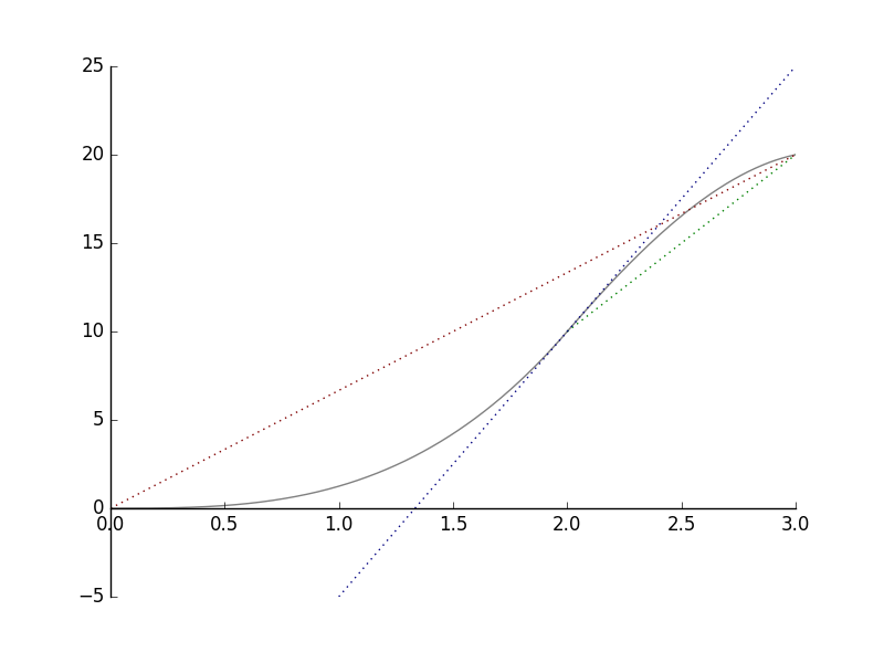
a) Look at the red line. We can see that in three hours, the cyclist moved  km. The average speed of the whole trip is
  km/h.
km/h.
b) Now look at the green line. We can see that during the third hour the cyclist moved  km further. That makes the average speed of that time interval km/h.
Notice that the slope of the red line is  and that the slope of the blue line is . These are the same values as the corresponding average speeds.
c) Look at the blue line. It is the tangent of the curve at the point  . Using the same principle as with average speeds, we conclude that after two hours of the departure, the speed of the cyclist was
  km/h
km/h  km/h.
km/h.
Now we will proceed to the general definition:
Definition: Derivative
Let \subset \mathbb{R}") . The derivative of function
. The derivative of function \to \mathbb{R}") at the point
at the point ") is
is :=\lim_{h\to 0} \frac{f(x_0+h)-f(x_0)}{h}.") If
If ") exists, then is said to be differentiable at the point .
exists, then is said to be differentiable at the point .
Note: Since  , then
  , and thus the definition can also be written in the form
 :=\lim_{x\to x_0} \frac{f(x)-f(x_0)}{x-x_0}.")
The derivative can be denoted in different ways: =Df(x_0) =\left. \frac{df}{dx}\right|_{x=x_0}, \ \ f'=Df =\frac{df}{dx}.")
Interpretation. Consider the curve ") . Now if we draw a line through the points
. Now if we draw a line through the points )") and
and )") , we see that the slope of this line is
, we see that the slope of this line is -f(x_0)}{x_0+h-x_0} = \frac{f(x_0+h)-f(x_0)}{h}.") When
When  , the line intersects with the curve only in the point
 )") . This line is the tangent of the curve
. This line is the tangent of the curve ") at the point and its slope is
at the point and its slope is -f(x_0)}{h},") which is the derivative of the function at
which is the derivative of the function at  . Hence, the tangent is given by the equation
 +f'(x_0)(x-x_0).")
Interactivity. Move the point of intersection and observe changes on the tangent line of the curve.
Example 1.
Let be the function  = x^3 + 1") . The derivative of at
. The derivative of at  is
is  &=\lim_{h \to 0} \frac{f(1+h)-f(1)}{h} \\ &=\lim_{h \to 0} \frac{(1+h)^3 + 1 - 1^3 - 1}{h} \\ &=\lim_{h \to 0} \frac{1+3h+3h^2+h^3-1}{h} \\ &=\lim_{h \to 0} \frac{h(3+3h+h^2)}{h} \\ &=\lim_{h \to 0} 3+3h+h^2 \\ &= 3. \end{aligned}")
Function  and its tangent at the point
  .
.
Example 2.
Let be the function =ax+b") . We find the derivative of .
. We find the derivative of .
Immediately from the definition we get: ![\begin{aligned}f'(x) &=\lim_{h\to 0} \frac{f(x+h)-f(x)}{h} \\ &=\lim_{h\to 0} \frac{[a(x+h)+b]-[ax+b]}{h} \\ &=\lim_{h\to 0} a \\ &=a.\end{aligned}](https://mycourses.aalto.fi/filter/tex/pix.php/5af936863c453fd1ea52d94c4e9b5344.gif "\begin{aligned}f'(x) &=\lim_{h\to 0} \frac{f(x+h)-f(x)}{h} \\ &=\lim_{h\to 0} \frac{[a(x+h)+b]-[ax+b]}{h} \\ &=\lim_{h\to 0} a \\ &=a.\end{aligned}")
Here is the slope of the tangent line. Note that the derivative at does not depend on because  is the equation of a line.
Note. When , we get  = b") and
and  = 0") . The derivative of a constant function is zero.
. The derivative of a constant function is zero.
Example 3.
Let  be the function
 =|x|") . Does have a derivative at ?
. Does have a derivative at ?
Now = \begin{cases}+1 & \text{when $x_{0}>0$} \\ -1 & \text{when $x_{0}")
The graph ") has no tangent at the point
has no tangent at the point  :
: -g(0)}{h}= \frac{|0+h|-|0|}{h}=\frac{|h|}{h}=\begin{cases}+1 & \text{for $h>0$}, \\ -1 & \text{for $h") Thus
Thus ") does not exist.
does not exist.
Conclusion. The function is not differentiable at the point .
Remark. Let . If ") exists for every
exists for every ") then we get a function
then we get a function \to \mathbb{R}") . We write:
. We write:
| (1) | |
= }(x)") , , |
|
| (2) | |
= }(x)") |
= ") , , |
| (3) | ") |
= }(x)") |
= ") , , |
| (4) | ") |
= }(x)") |
= ") , , |
| ... |
Here is called the second derivative of at , }") is the third derivative, and so on.
is the third derivative, and so on.
We introduce the notation \begin{eqnarray} C^n\bigl( ]a,b[\bigr) =\{ f\colon \, ]a,b[\, \to \mathbb{R} & \mid & f \text{ is } n \text{ times differentiable on the interval } ]a,b[ \nonumber \\ & & \text{ and } f^{(n)} \text{ is continuous}\}. \nonumber \end{eqnarray} These functions are said to be n times continuously differentiable.
Function .
Example 4.
The distance moved by a cyclist (or a car) is given by ") . Then the speed at the moment
. Then the speed at the moment  is
is ") and the acceleration is
and the acceleration is ") .
.
Linearization and differential
\approx \frac{f(x)-f(x_0)}{x-x_0} \Leftrightarrow f(x)\approx f(x_0)+f'(x_0)(x-x_0),") where the right-handed side is the linearization or the differential of at . The differential is denoted by
where the right-handed side is the linearization or the differential of at . The differential is denoted by  . The graph of the linearization,
 +f'(x_0)(x-x_0),") is the tangent line drawn on the graph of the function at the point . Later, in multi-variable calculus, the true meaning of the differential becomes clear. For now, it is not necessary to get troubled by the details.
is the tangent line drawn on the graph of the function at the point . Later, in multi-variable calculus, the true meaning of the differential becomes clear. For now, it is not necessary to get troubled by the details.
Properties of derivative
Next we give some useful properties of the derivative. These properties allow us to find derivatives for some familiar classes of functions such as polynomials and rational functions.
Continuity and derivative
If is differentiable at the point , then is continuous at the point :  = f(x_0).") Why? Because if is differentiable, then we get
Why? Because if is differentiable, then we get +h\frac{f(x_0+h)-f(x_0)}{h} \rightarrow f(x_0)+0\cdot f'(x_0)=f(x_0),") as .
as .
Note. If a function is continuous at the point , it doesn't have to be differentiable at that point. For example, the function  = |x|") is continuous, but not differentiable at the point .
is continuous, but not differentiable at the point .
Differentiation Rules
Next we will give some important rules which are often applied in practical problems concerning determination of the derivative of a given function.
Suppose that and are differentiable at .
A Constant Multiplier
'(x) = cf'(x),\ c \in \mathbb{R}")
Suppose that is differentiable at . We determine: '(x),") where is a constant.
where is a constant.
(x+h)-(cf)(x)}{h} \ & \ = \ \frac{cf(x+h)-cf(x)}{h} \\ & \ = \ c \ \frac{f(x+h)-f(x)}{h}\end{aligned}")
As  , we get
 -f(x)}{h} \to c f'(x).")
The Sum Rule
'(x) = f'(x) + g'(x)")
'(x).")
![\begin{aligned}\frac{(f+g)(x+h)-(f+g)(x)}{h} \ & \ = \ \frac{[f(x+h)+g(x+h)]-[f(x)+g(x)]}{h} \\ & \ = \ \frac{f(x+h)-f(x)}{h}+\frac{g(x+h)-g(x)}{h}\end{aligned}](https://mycourses.aalto.fi/filter/tex/pix.php/ef8575955c1913eb61f3bda0de6c3ee8.gif "\begin{aligned}\frac{(f+g)(x+h)-(f+g)(x)}{h} \ & \ = \ \frac{[f(x+h)+g(x+h)]-[f(x)+g(x)]}{h} \\ & \ = \ \frac{f(x+h)-f(x)}{h}+\frac{g(x+h)-g(x)}{h}\end{aligned}")
-f(x)}{h}+\frac{g(x+h)-g(x)}{h}\to \ f'(x)+g'(x)")
The Product Rule
'(x) = f'(x)g(x) + f(x)g'(x)")
Suppose that  and are differentiable at . We determine
 '(x).")
(x+h)-(fg)(x)}{h} & = \frac{f(x+h)g(x+h)-f(x)g(x)}{h} \\ & = \frac{f(x+h)g(x+h)-f(x)g(x+h)+f(x)g(x+h)-f(x)g(x)}{h} \\ & = \frac{f(x+h)-f(x)}{h}\ g(x+h)+f(x)\ \frac{g(x+h)-g(x)}{h}\end{aligned}")
When , we get -f(x)}{h}g(x+h)+f(x)\frac{g(x+h)-g(x)}{h}\to f'(x)g(x)+f(x)g'(x).")
The Power Rule

For  we repeteadly apply the product rule, and obtain
  \\ & = (\frac{d}{dx}x)x^{n-1}+x\frac{d}{dx}x^{n-1} \\ & \stackrel{dx/dx=1}{=} x^{n-1}+x\frac{d}{dx}x^{n-1} \\ & = x^{n-1}+x\left( x^{n-2}+x\frac{d}{dx}x^{n-2}\right) \\ & = \ldots \\ & = \sum_{k=0}^{n-1} x^{n-1} \\ & = nx^{n-1}.\end{aligned}")
The case of negative  is obtained from this and the product rule applied to the identity
  .
.
From the power rule we obtain a formula for the derivative of a polynomial. Let =a_n x^{n}+a_{n-1}x^{n-1}+\ldots+ a_1 x + a_0,") where . Then
where . Then =na_nx^{n-1}+(n-1)a_{n-1}x^{n-2}+\ldots +2 a_2 x+a_1.")
The Reciprocal Rule
'(x) = - \frac{f'(x)}{f(x)^2} \text{, } f(x) \neq 0")
Suppose that is differentiable at and \neq 0") . We determine
. We determine '(x).")
From the definition we obtain: (x+h)-(1/f)(x)}{h} & = \frac{1/f(x+h)-1/f(x)}{h} \\ & = \frac{\frac{f(x)}{f(x)f(x+h)}-\frac{f(x+h)}{f(x)f(x+h)}}{h} \\ & = \frac{f(x)-f(x+h)}{h}\frac{1}{f(x)f(x+h)}\end{aligned}")
Because is differentiable at we get -f(x+h)}{h}\frac{1}{f(x)f(x+h)}=-f'(x)/f(x)^2,") as .
as .
The Quotient Rule
'(x) = \frac{f'(x)g(x)-f(x)g'(x)}{g(x)^2},\ g(x) \neq 0")
Suppose that are differentiable at and \neq 0") . Then
. Then '(x) & = \Big( f \cdot \frac{1}{g}\Big) '(x) \\ & = f'(x)\frac{1}{g(x)}-f(x)\frac{g'(x)}{g(x)^2} \\ & = \frac{f'(x)g(x)-f(x)g'(x)}{g(x)^2}.\end{aligned}")
Interactivity. Vary and the constant multiplier and see the effect of constant multiplier rule in practice.
Example 1.
=\frac{d}{dx}x^{2006}+5\frac{d}{dx}x^3+42\frac{d}{dx}1=2006x^{2005}+5\cdot 3x^2.")
Example 2.
![\begin{aligned}\frac{d}{dx} [(x^4-2)(2x+1)] &= \frac{d}{dx}(x^4-2) \cdot (2x+1) + (x^4-2) \cdot \frac{d}{dx}(2x + 1) \\ &= 4x^3(2x+1) + 2(x^4-2) \\ &= 8x^4+4x^3+2x^4-4 \\ &= 10x^4+4x^3-4.\end{aligned}](https://mycourses.aalto.fi/filter/tex/pix.php/8c708f0f3c9ec809601fbd059363c2b4.gif "\begin{aligned}\frac{d}{dx} [(x^4-2)(2x+1)] &= \frac{d}{dx}(x^4-2) \cdot (2x+1) + (x^4-2) \cdot \frac{d}{dx}(2x + 1) \\ &= 4x^3(2x+1) + 2(x^4-2) \\ &= 8x^4+4x^3+2x^4-4 \\ &= 10x^4+4x^3-4.\end{aligned}")
Note. We can check the answer by deriving it in another way: ![\frac{d}{dx} [(x^4-2)(2x+1)] = \frac{d}{dx} (2x^5 +x^4 -4x -2) = 10x^4 +4x^3 -4.](https://mycourses.aalto.fi/filter/tex/pix.php/d030d685c2973158b90ad35a97a50d5b.gif "\frac{d}{dx} [(x^4-2)(2x+1)] = \frac{d}{dx} (2x^5 +x^4 -4x -2) = 10x^4 +4x^3 -4.")
Function (2x+1)") .
.
Example 3.
For  we get
 ^2} = -3 \cdot \frac{3x^2}{x^6}= - \frac{9}{x^4}.")
Note. There is another way of solving the problem above by noticing that  and differentiating it as a power:
 = - \frac{9}{x^4}")
Example 4.
(1+x^2)-x^3\frac{d}{dx}(1+x^2)}{(1+x^2)^2} \\ & = \frac{3x^2(1+x^2)-x^3(2x)}{(1+x^2)^2} \\ & = \frac{3x^2+x^4}{(1+x^2)^2}.\end{aligned}")
Function ") .
.
Rolle's Theorem
If is differentiable at a local extremum ![x_0\in \, ]a,b[](https://mycourses.aalto.fi/filter/tex/pix.php/b4b89672d69ecf8369f43f7dd31f0d2c.gif "x_0\in \, ]a,b[") , then
, then =0") .
.
The one-sided limits of the difference quotient have different signs at a local extremum. For example, for a local maximum it holds that \begin{eqnarray} \frac{f(x_0+h)-f(x_0)}{h} = \frac{\text{negative} }{\text{positive}}&\le& 0, \text{ when } h>0, \nonumber \\ \frac{f(x_0+h)-f(x_0)}{h} = \frac{\text{negative}}{\text{negative}}&\ge& 0, \text{ when } h<0 \nonumber \end{eqnarray} and  is so small that is a maximum on the interval
 ![[x_0-h,x_0+h]](https://mycourses.aalto.fi/filter/tex/pix.php/fa82e5aaac1e1a7465724ab32e282839.gif "[x_0-h,x_0+h]") .
.
L'Hospital's Rule
There are many different versions of this rule, but we present only the simplest one. Let us assume that =g(x_0)=0") and the functions are differentiable on some interval
and the functions are differentiable on some interval ![]x_0-\delta,x_0+\delta[](https://mycourses.aalto.fi/filter/tex/pix.php/c9bd44b465175498c9476b6701b55fca.gif "]x_0-\delta,x_0+\delta[") . If
. If }{g'(x)}") exists, then
exists, then }{g(x)}=\lim_{x\to x_0}\frac{f'(x)}{g'(x)}.")
In the special case \neq 0") the proof is simple:
the proof is simple: }{g(x)}=\frac{f(x)-f(x_0)}{g(x)-g(x_0)} = \frac{\bigl( f(x)-f(x_0)\bigr) /(x-x_0)}{\bigl( g(x)-g(x_0)\bigr) /(x-x_0)} \to \frac{f'(x_0)}{g'(x_0)}.") In the general case we need the so-called generalized mean value theorem, which states that
In the general case we need the so-called generalized mean value theorem, which states that }{g(x)} = \frac{f'(c)}{g'(c)}") for some
for some ![c\in \, ]x_0,x[](https://mycourses.aalto.fi/filter/tex/pix.php/5c97c28ce97d3f291e533efe3f450068.gif "c\in \, ]x_0,x[") . Here we have the same point
. Here we have the same point  both in the numerator and the denominator, so we do not even need the continuity of the derivatives!
Derivatives of Trigonometric Functions
In this section, we give differentiation formulas for trigonometric functions  ,
,  and
and  .
.
Derivative of Sine
=\cos(t)")
")
![\begin{aligned}\sin'(t) & = \lim_{h\to 0} \frac{\sin(t+h)-\sin(t)}{h} \\
& = \lim_{h\to 0} \frac{[\sin(t)\cos(h)+\cos(t)\sin(h)]-\sin(t)}{h} \\
& = \lim_{h\to 0}\sin(t)\frac{\cos(h)-1}{h}+\lim_{h\to 0}\cos(t)\frac{\sin(h)}{h}.
\end{aligned}](https://mycourses.aalto.fi/filter/tex/pix.php/43dab0c7e1606d265f8428433a47b025.gif "\begin{aligned}\sin'(t) & = \lim_{h\to 0} \frac{\sin(t+h)-\sin(t)}{h} \\
& = \lim_{h\to 0} \frac{[\sin(t)\cos(h)+\cos(t)\sin(h)]-\sin(t)}{h} \\
& = \lim_{h\to 0}\sin(t)\frac{\cos(h)-1}{h}+\lim_{h\to 0}\cos(t)\frac{\sin(h)}{h}.
\end{aligned}")

} =
-\frac{\sin h}{h}\cdot \frac{\sin h}{\cos h+1} \to -1\cdot 0 = 0")

=\cos(t).")
Function ") and its derivative function
and its derivative function ") .
.
Derivative of Cosine
= - \sin(t)")
This follows in a similar way as the derivative of Sine, but more easily from the identity =\sin(\pi/2-t)") and the Chain rule to be introduced in the following section.
and the Chain rule to be introduced in the following section.
Function and its derivative function ") .
.
 = \frac{1}{\cos^2(t)}=1+\tan^2 t.")
=\frac{\sin(t)}{\cos(t)},")
=\frac{\sin'(t)\cos(t)-\sin(t)\cos'(t)}{\cos^2(t)}=\frac{\cos^2(t)+\sin^2(t)}{\cos^2(t)}=\begin{cases}\frac{1}{\cos^2(t)} & \\ 1+\tan^2 t.\end{cases}")
Function and its derivative function ") .
.
Example 1.
) = 3 \sin'(x) = 3 \cos(x).")
Example 2.
 = \cos'(x) \cdot \cos(x) + \cos(x) \cdot \cos'(x) = -2\sin(x)\cos(x).")
Example 3.
 + 1}{\cos(x)} &= \frac{d}{dx} \left( \frac{\sin(x)}{\cos(x)} + \frac{1}{\cos(x)} \right) \\
&= \tan'(x) - \frac{\cos'(x)}{\cos^2(x)} \\
&= \frac{1+\sin(x)}{\cos^2 (x)}.\end{aligned}")
The Chain Rule
In this section we learn a formula for finding the derivative of a composite function. This important formula is known as the Chain Rule.
The Chain Rule.
Let  , and
, and  .
.
Let be differentiable at the point and at ") . Then
. Then
)=f'(g(x))g'(x).")
Consider
)-f(g(x))}{h} &= \frac{f(g(x+h))-f(g(x))}{h} \ \frac{g(x+h)-g(x)}{g(x+h)-g(x)} \\
&= \frac{f(g(x+h))-f(g(x))}{g(x+h)-g(x)} \ \frac{g(x+h)-g(x)}{h}.\end{aligned}")
Now let us write :=g(x+h)-g(x)") . Then
. Then =g(x)+k(h)") and we get
and we get
)-f(g(x))}{h}=\frac{f(g(x)+k(h))-f(g(x))}{k(h)}\frac{g(x+h)-g(x)}{h}.")
Problem. What if =0") ? Note that one cannot divide by zero.
? Note that one cannot divide by zero.
Solution. Define
:= \begin{cases}0, & \text{for $k=0$}, \\
\frac{f(g(x)+k)-f(g(x))}{k}-f'(g(x)), & \text{for $k\neq 0$},\end{cases}") so that
so that
![\frac{f(g(x+h))-f(g(x))}{h}=[E(k(h))+f'(g(x))]\frac{g(x+h)-g(x)}{h}.](https://mycourses.aalto.fi/filter/tex/pix.php/4772424382ad3806e0cca96db8c05fd1.gif "\frac{f(g(x+h))-f(g(x))}{h}=[E(k(h))+f'(g(x))]\frac{g(x+h)-g(x)}{h}.") Now, because
Now, because  is continuous, we get
![[E(k(h))+f'(g(x))]\frac{g(x+h)-g(x)}{h}\to f'(g(x))g'(x).](https://mycourses.aalto.fi/filter/tex/pix.php/57e9195f36e9ff554cd408a7b174bd50.gif "[E(k(h))+f'(g(x))]\frac{g(x+h)-g(x)}{h}\to f'(g(x))g'(x).") as .
as .
Example 1.
The problem is to differentiate the function ^3") . We take
. We take  = x^3") and
and  = 2x-1") and differentiate the composite function
and differentiate the composite function )") . As
. As
 = 3x^2 \text{ and } g'(x) = 2,") we get
we get
^3 = 3(2x-1)^2 \cdot 2 = 6(4x^2-4x+1) = 24x^2-24x+6.")
Function and its derivative function.
Example 2.
We need to differentiate the function  . Take
  = \sin x") and
and  = 3x") , then differentiate the composite function .
, then differentiate the composite function .

Remark. Let  and . Now
))=f'(g(h(x)))\frac{d}{dx}g(h(x))=f'(g(h(x)))g'(h(x))h'(x).") Similarly, one may obtain even more complex rules for composites of multiple functions.
Similarly, one may obtain even more complex rules for composites of multiple functions.
Function and its derivative function.
Example 3.
Differentiate the function  . Take ,
  = \cos x") and
and  = 2x") and differentiate the composite function
and differentiate the composite function ))") .
.
^2 \cdot \frac{d}{dx} \cos 2x \\
&= 3 \cos^2 2x \cdot (-\sin 2x) \cdot 2 \\
&= -6 \sin 2x \cos^2 2x.\end{aligned}")
Function and its derivative function.
Extremal Value Problems
We will discuss the Intermediate Value Theorem for differentiable functions, and its connections to extremal value problems.
Definition: Local Maxima and Minima
A function  has a a local maximum at the point
  , if for some
  and for all
  such that
  , we have
 \leq f(x_0)") .
.
Similarly, a function has a local minimum at the point , if for some  and for all such that , we have
 \geq f(x_0)") .
.
A local extreme is a local maximum or a local minimum.
Remark. If is a local maximum value and exists, then
 & =\lim_{h\to 0^{+}}\frac{f(x_0+h)-f(x_0)}{h} \leq 0 \\
f'(x_0) & =\lim_{h\to 0^{-}}\frac{f(x_0+h)-f(x_0)}{h} \geq 0.\end{cases}") Hence .
Hence .
We get:
Theorem 1.
Let ![x_0\in [a,b]](https://mycourses.aalto.fi/filter/tex/pix.php/f1f8b7afdbcc5f31096799e43c43711e.gif "x_0\in [a,b]") be a local extremal value of a continuous function . Then either
be a local extremal value of a continuous function . Then either
the derivative
doesn't exist (this includes also cases  and
and  ) or
) or- .
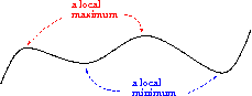
Example 1.
Let be defined by
 = x^3 -3x + 1.") Then
Then
 = 3x^2-3") and we can see that at the points
and we can see that at the points  and the local maximum and minimum of are obtained,
 = 3 \cdot (-1)^2 - 3 = 0 \text{ and } f'(1) = 3 \cdot 1^2 - 3 = 0.")
Function  and its derivative function
  .
.
Finding the global extrema
In practice, when we are looking for the local extrema of a given function, we need to check three kinds of points:
the zeros of the derivative
the endpoints of the domain of definition (interval)
points where the function is not differentiable
If we happened to know beforehand that the function has a minimum/maximum, then we start off by finding all the possible local extrema (the points described above), evaluate the function at these points and pick the greatest/smallest of these values.
Example 2.
Let us find the smallest and greatest value of the function ![f\colon [0,2]\to \mathbf{R}](https://mycourses.aalto.fi/filter/tex/pix.php/ee77c8a9721b9494f327d61422eb2068.gif "f\colon [0,2]\to \mathbf{R}") ,
, =x^3-6x") . Since the function is continuous on a closed interval, then it has a maximum and a minimum. Since the function is differentiable, it is sufficient to examine the endpoints of the interval and the zeros of the derivative that are contained in the interval.
. Since the function is continuous on a closed interval, then it has a maximum and a minimum. Since the function is differentiable, it is sufficient to examine the endpoints of the interval and the zeros of the derivative that are contained in the interval.
The zeros of the derivative: =3x^2-6=0 \Leftrightarrow x=\pm \sqrt{2}") .
Since
.
Since ![-\sqrt{2}\not\in [0,2]](https://mycourses.aalto.fi/filter/tex/pix.php/601d5044bf746b9e7af4678c2c3463a1.gif "-\sqrt{2}\not\in [0,2]") , we only need to evaluate the function at three points,
, we only need to evaluate the function at three points, =0") ,
, =-4\sqrt{2}") and
and =-4") . From these we can see that the smallest value of the function is
. From these we can see that the smallest value of the function is  and the greatest value is , respectively.
Next we will formulate a fundamental result for differentiable functions. The basic idea here is that the change on an interval can only happen, if there is change at some point on the inverval.
Theorem 2.
(The Intermediate Value Theorem for Differentiable Functions). Let be continuous in the interval and differentiable in the interval ") . Then
. Then
=\frac{f(b)-f(a)}{b-a}") for some
for some .")
Let be continuous in the interval and differentiable in the interval . Let us define
:=f(x)-\frac{f(b)-f(a)}{b-a}(x-a)-f(a).")
Now =g(b)=0") and is differentiable in the interval . According to Rolle's Theorem, there exists
and is differentiable in the interval . According to Rolle's Theorem, there exists ") such that
such that =0") . Hence
. Hence
=g'(c)+\frac{f(b)-f(a)}{b-a}=\frac{f(b)-f(a)}{b-a}.")
This result has an important application:
Theorem 3.
Let be a differentiable function. Then
If for all
 \ \ f'(x)\geq 0") , then is increasing,
, then is increasing,If for all
 \ \ f'(x)\leq 0") , then is decreasing.
, then is decreasing.
Suppose that  .
.
Then by Theorem 2 there exists ") such that
such that
=\frac{f(x_2)-f(x_1)}{x_2-x_1}.")
It follows that -f(x_1)=f'(x_0)(x_2-x_1)") .
.
Hence we may conclude that is increasing for \geq 0") and decreasing for
and decreasing for \leq 0") .
.
Example 3.
For the polynomial  = \frac{1}{4} x^4-2x^2-7") the derivative is
the derivative is
 = x^3-4x = x(x^2-4) = 0,") when ,
when ,  or
or  . Now we can draw a table:
|
 |
 |
 |
|
|---|---|---|---|---|
|
 |
|
 |
|
 |
|
|
|
|
|
|
|
|
|
|
decr. | incr. | decr. | incr. |
Function  .
.
Example 4.
We need to find a rectangle so that its area is  and it has the least possible perimeter.
Let ") and
and ") be the sides of the rectangle. Then
be the sides of the rectangle. Then  and we get
  . Now the perimeter is
 In which point does the function
  = \frac{2x^2+18}{x}") get its minimum value? Function is continuous and differentiable, when and using the quotient rule, we get
get its minimum value? Function is continuous and differentiable, when and using the quotient rule, we get
 = \frac{4x \cdot x-(2x^2+18) \cdot 1}{x^2} = \frac{2x^2-18}{x^2}.") Now , when
Now , when
 but we have defined that and therefore are only interested in the case
  . Let's draw a table:
|
 |
|
|---|---|---|
|
|
|
|
decr. | incr. |
As the function is continuous, we now know that it attains its minimum at the point . Now we calculate the other side of the rectangle:  .
.
Thus, the rectangle, which has the least possible perimeter is actually a square, which sides are of the length  .
.
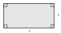
Function  .
.
Example 5.
We must make a one litre measure, which is shaped as a right circular cylinder without a lid. The problem is to find the best size of the bottom and the height so that we need the least possible amount of material to make the measure.
Let  be the radius and
  the height of the cylinder. The volume of the cylinder is dm
 and we can write
  from which we get

The amount of material needed is the surface area

Let function  \to \mathbb{R}") be defined by
be defined by
 = \pi r^2 + \frac{2}{r}.") We must find the minimum value for function , which is continuous and differentiable, when
We must find the minimum value for function , which is continuous and differentiable, when  . Using the reciprocal rule, we get
 = 2\pi r -2 \cdot \frac{1}{r^2} = \frac{2\pi r^3 - 2}{r^2}.") Now
Now  = 0") , when
, when
![\begin{aligned}2\pi r^3 - 2 &= 0 \\
2\pi r^3 &= 2 \\
r^3 &= \frac{1}{\pi} \\
r &= \frac{1}{\sqrt[3]{\pi}}.\end{aligned}](https://mycourses.aalto.fi/filter/tex/pix.php/ffb8cf82115510a023a5408e30bf2b57.gif "\begin{aligned}2\pi r^3 - 2 &= 0 \\
2\pi r^3 &= 2 \\
r^3 &= \frac{1}{\pi} \\
r &= \frac{1}{\sqrt[3]{\pi}}.\end{aligned}")
Let's draw a table:
 |
![r>\frac{1}{\sqrt[3]{\pi}}](https://mycourses.aalto.fi/filter/tex/pix.php/70296efeaa006fb5cd9c2f29b5d0a0e2.gif "r>\frac{1}{\sqrt[3]{\pi}}") |
|
|---|---|---|
") |
|
|
") |
decr. | incr. |
As the function is continuous, we now know that it gets its minimum value at the point ![r= \frac{1}{\sqrt[3]{\pi}} \approx 0.683](https://mycourses.aalto.fi/filter/tex/pix.php/ef4b63276241174d0f518a6b4301d081.gif "r= \frac{1}{\sqrt[3]{\pi}} \approx 0.683") . Then
. Then
![h = \frac{1}{\pi r^2} = \frac{1}{\pi \left(\frac{1}{\sqrt[3]{\pi}}\right)^2} = \frac{1}{\frac{\pi}{\pi^{2/3}}} = \frac{1}{\sqrt[3]{\pi}} \approx 0.683.](https://mycourses.aalto.fi/filter/tex/pix.php/8af221027cf46db4d652e5781ac056d2.gif "h = \frac{1}{\pi r^2} = \frac{1}{\pi \left(\frac{1}{\sqrt[3]{\pi}}\right)^2} = \frac{1}{\frac{\pi}{\pi^{2/3}}} = \frac{1}{\sqrt[3]{\pi}} \approx 0.683.")
This means that it would take least materials to make a measure, which is approximately  dm
dm  dm
dm  cm in diameter and
  dm
dm  cm high.

Function  .
.
',
label : { strokeColor : 'blue' }
});
var t = board.create('tangent', [g1], {
strokeWidht : 2,
strokeOpacity : .8
});
var text1 = board.create('text', [-4, 5, function() { return ' = x^3+2x^2") '}], {
useMathJax : true,
fontSize : 14,
strokeColor : 'black'
});
var text2 = board.create('text', [-4, 4, function() {
var k = t.getSlope();
var b = g1.Y()-k*g1.X();
var temp = '';
if(k == 0) {
temp = '
'}], {
useMathJax : true,
fontSize : 14,
strokeColor : 'black'
});
var text2 = board.create('text', [-4, 4, function() {
var k = t.getSlope();
var b = g1.Y()-k*g1.X();
var temp = '';
if(k == 0) {
temp = ' +'") ';
} else {
if(b < 0) {
temp = '
';
} else {
if(b < 0) {
temp = ' + 'x' + b.toFixed(2) + '") ';
} else {
temp = '
';
} else {
temp = ' + 'x + ' + b.toFixed(2) + '") ';
}
}
return temp;
}
], {
useMathJax : true,
fontSize : 14,
strokeColor : 'blue'
});
})();
(function() {
var board = JXG.JSXGraph.initBoard('jxgbox03', {
boundingbox : [-3.5, 3, 3.5, -3],
axis : false,
shownavigation : false,
showcopyright : false
});
var xaxis = board.create('axis', [[0, 0],[1, 0]], {
ticks : { majorHeight : 5 }
});
var yaxis = board.create('axis' ,[[0, 0],[0, 1]], {
ticks : { majorHeight : 5}
});
var f = function(x) { return x*x*x+1; }
var graph = board.create('functiongraph', [f, -3.5, 3.5], {
strokeWidth : 1.5,
strokeColor : 'black'
});
var g1 = board.create('glider', [1, f(1), graph], { strokeColor : 'black', size : 2, fillColor : 'red', name : '' });
var t = board.create('tangent', [g1], { strokeColor : 'red', strokeWidth : 1.5 });
var a = board.create('segment', [[function() { return g1.X() }, function() { return g1.Y()-t.getSlope(); }],
[function() { return g1.X()-1; }, function() { return g1.Y()-t.getSlope() }]], {
strokeWidth : 2,
strokeOpacity : .8,
dash : 1,
highlight : false
});
var b = board.create('segment', [[ function() { return g1.X(); }, function() { return g1.Y(); }],
[ function() { return a.point1.X(); }, function() { return a.point1.Y(); } ]], {
strokeWidth : 2,
strokeOpacity : .8,
dash : 1,
highlight : false
});
})();
(function() {
var board = JXG.JSXGraph.initBoard('jxgbox04', {
boundingbox : [-5, 5, 5, -2],
axis : false,
shownavigation : false,
showcopyright : false
});
var xaxis = board.create('axis', [[0, 0], [1, 0]], {
highlight : false,
drawZero : true,
ticks : { minorTicks : 0, majorHeight : 9, label : { highlight : false, offset : [-5, -15] } }
});
var yaxis = board.create('axis', [[0, 0], [0, 1]], {
highlight : false,
ticks : { minorTicks : 0, majorHeight : 9, label : { offset : [-15, 0 ], position : 'lrt', highlight : false } }
});
xaxis.defaultTicks.ticksFunction = function() { return 1; };
yaxis.defaultTicks.ticksFunction = function() { return 1; };
var f = function(x) { return Math.abs(x); }
board.create('functiongraph', [f, -5, 5], {
strokeWidth : 2,
strokeColor : '#2183de',
highlight : false
});
board.create('text', [1.5, 1.2, function() { return '
';
}
}
return temp;
}
], {
useMathJax : true,
fontSize : 14,
strokeColor : 'blue'
});
})();
(function() {
var board = JXG.JSXGraph.initBoard('jxgbox03', {
boundingbox : [-3.5, 3, 3.5, -3],
axis : false,
shownavigation : false,
showcopyright : false
});
var xaxis = board.create('axis', [[0, 0],[1, 0]], {
ticks : { majorHeight : 5 }
});
var yaxis = board.create('axis' ,[[0, 0],[0, 1]], {
ticks : { majorHeight : 5}
});
var f = function(x) { return x*x*x+1; }
var graph = board.create('functiongraph', [f, -3.5, 3.5], {
strokeWidth : 1.5,
strokeColor : 'black'
});
var g1 = board.create('glider', [1, f(1), graph], { strokeColor : 'black', size : 2, fillColor : 'red', name : '' });
var t = board.create('tangent', [g1], { strokeColor : 'red', strokeWidth : 1.5 });
var a = board.create('segment', [[function() { return g1.X() }, function() { return g1.Y()-t.getSlope(); }],
[function() { return g1.X()-1; }, function() { return g1.Y()-t.getSlope() }]], {
strokeWidth : 2,
strokeOpacity : .8,
dash : 1,
highlight : false
});
var b = board.create('segment', [[ function() { return g1.X(); }, function() { return g1.Y(); }],
[ function() { return a.point1.X(); }, function() { return a.point1.Y(); } ]], {
strokeWidth : 2,
strokeOpacity : .8,
dash : 1,
highlight : false
});
})();
(function() {
var board = JXG.JSXGraph.initBoard('jxgbox04', {
boundingbox : [-5, 5, 5, -2],
axis : false,
shownavigation : false,
showcopyright : false
});
var xaxis = board.create('axis', [[0, 0], [1, 0]], {
highlight : false,
drawZero : true,
ticks : { minorTicks : 0, majorHeight : 9, label : { highlight : false, offset : [-5, -15] } }
});
var yaxis = board.create('axis', [[0, 0], [0, 1]], {
highlight : false,
ticks : { minorTicks : 0, majorHeight : 9, label : { offset : [-15, 0 ], position : 'lrt', highlight : false } }
});
xaxis.defaultTicks.ticksFunction = function() { return 1; };
yaxis.defaultTicks.ticksFunction = function() { return 1; };
var f = function(x) { return Math.abs(x); }
board.create('functiongraph', [f, -5, 5], {
strokeWidth : 2,
strokeColor : '#2183de',
highlight : false
});
board.create('text', [1.5, 1.2, function() { return '=|x|") '; }], {
useMathJax : true,
strokeColor : '#2183de',
fontSize : 13,
fixed : true,
highlight : false
});
board.fullUpdate();
})();
(function() {
var board = JXG.JSXGraph.initBoard('jxgbox05', {
boundingbox : [-1.7, 10.1, 1.7, -10.1],
axis : false,
shownavigation : false,
showcopyright : false
});
var xaxis = board.create('axis', [[0, 0], [1, 0]], {
highlight : false,
drawZero : true,
ticks : { minorTicks : 0, majorHeight : 9, label : { highlight : false, offset : [-5, -15] } }
});
var yaxis = board.create('axis', [[0, 0], [0, 1]], {
highlight : false,
ticks : { minorTicks : 0, majorHeight : 9, label : { offset : [-15, 0 ], position : 'lrt', highlight : false } }
});
xaxis.defaultTicks.ticksFunction = function() { return 1; };
yaxis.defaultTicks.ticksFunction = function() { return 5; };
var f = function(x) { return (x*x*x*x-2)*(2*x+1); }
board.create('functiongraph', [f, -1.7, 1.7], {
strokeWidth : 2.5,
strokeColor : 'black',
highlight : false
});
board.fullUpdate();
})();
(function() {
var board = JXG.JSXGraph.initBoard('jxgbox06', {
boundingbox : [-6.1, 6.5, 6.1, -6.5],
axis : false,
shownavigation : false,
showcopyright : false
});
var xaxis = board.create('axis', [[0, 0], [1, 0]], {
highlight : false,
drawZero : true,
ticks : { minorTicks : 0, majorHeight : 9, label : { highlight : false, offset : [-5, -15] } }
});
var yaxis = board.create('axis', [[0, 0], [0, 1]], {
highlight : false,
ticks : { minorTicks : 0, majorHeight : 9, label : { offset : [-15, 0 ], position : 'lrt', highlight : false } }
});
xaxis.defaultTicks.ticksFunction = function() { return 2; };
yaxis.defaultTicks.ticksFunction = function() { return 2; };
var f = function(x) { return x*x*x/(1+x*x); }
board.create('functiongraph', [f, -6.1, 6.1], {
strokeWidth : 2.5,
strokeColor : 'black',
highlight : false
});
board.fullUpdate();
})();
(function() {
var board = JXG.JSXGraph.initBoard('jxgbox07', {
boundingbox : [-6.77, 6, 6.77, -6],
axis : false,
shownavigation : false,
showcopyright : false
});
var xaxis = board.create('axis', [[0, 0], [1, 0]], {
highlight : false,
drawZero : true,
ticks : { minorTicks : 0, majorHeight : 9, label : { highlight : false, offset : [-5, -15] } }
});
var yaxis = board.create('axis', [[0, 0], [0, 1]], {
highlight : false,
ticks : { minorTicks : 0, majorHeight : 9, label : { offset : [-15, 0 ], position : 'lrt', highlight : false } }
});
var f = function(x) { return Math.sin(x); }
var df = function(x) { return Math.cos(x); }
board.create('functiongraph', [f, -6.77, 6.77], {
strokeWidth : 1.5,
strokeColor : 'red'
});
board.create('functiongraph', [df, -6.77, 6.77], {
strokeWidth : 1.5,
strokeColor : 'black'
});
})();
(function() {
var board = JXG.JSXGraph.initBoard('jxgbox08', {
boundingbox : [-6.77, 6, 6.77, -6],
axis : false,
shownavigation : false,
showcopyright : false
});
var xaxis = board.create('axis', [[0, 0], [1, 0]], {
highlight : false,
drawZero : true,
ticks : { minorTicks : 0, majorHeight : 9, label : { highlight : false, offset : [-5, -15] } }
});
var yaxis = board.create('axis', [[0, 0], [0, 1]], {
highlight : false,
ticks : { minorTicks : 0, majorHeight : 9, label : { offset : [-15, 0 ], position : 'lrt', highlight : false } }
});
var f = function(x) { return Math.cos(x); }
var df = function(x) { return Math.sin(x); }
board.create('functiongraph', [f, -6.77, 6.77], {
strokeWidth : 1.5,
strokeColor : 'blue'
});
board.create('functiongraph', [df, -6.77, 6.77], {
strokeWidth : 1.5,
strokeColor : 'black'
});
})();
(function() {
var board = JXG.JSXGraph.initBoard('jxgbox09', {
boundingbox : [-6.77, 6, 6.77, -6],
axis : false,
shownavigation : false,
showcopyright : false
});
var xaxis = board.create('axis', [[0, 0], [1, 0]], {
highlight : false,
drawZero : true,
ticks : { minorTicks : 0, majorHeight : 9, label : { highlight : false, offset : [-5, -15] } }
});
var yaxis = board.create('axis', [[0, 0], [0, 1]], {
highlight : false,
ticks : { minorTicks : 0, majorHeight : 9, label : { offset : [-15, 0 ], position : 'lrt', highlight : false } }
});
var f = function(x) { return Math.tan(x); }
var df = function(x) { return 1/Math.pow(Math.cos(x),2); }
board.create('functiongraph', [f, -6.77, 6.77], {
strokeWidth : 1.5,
strokeColor : 'green'
});
board.create('functiongraph', [df, -6.77, 6.77], {
strokeWidth : 1.5,
strokeColor : 'black'
});
})();
(function() {
var board = JXG.JSXGraph.initBoard('jxgbox10', {
boundingbox : [-3.2, 4.5, 4.8, -2.5],
axis : false,
shownavigation : false,
showcopyright : false
});
var xaxis = board.create('axis', [[0, 0], [1, 0]], {
highlight : false,
drawZero : true,
ticks : { minorTicks : 0, majorHeight : 9, label : { highlight : false, offset : [-5, -15] } }
});
var yaxis = board.create('axis', [[0, 0], [0, 1]], {
highlight : false,
ticks : { minorTicks : 0, majorHeight : 9, label : { offset : [-15, 0 ], position : 'lrt', highlight : false } }
});
var f = function(x) { return Math.pow(2*x*x-1, 3); }
var df = function(x) { return 6*Math.pow(2*x*x-1, 2); }
board.create('functiongraph', [f, 0, 4.8], {
strokeWidth : 1.5,
strokeColor : 'green'
});
board.create('functiongraph', [df, 0, 4.8], {
strokeWidth : 1.5,
strokeColor : 'black'
});
})();
(function() {
var board = JXG.JSXGraph.initBoard('jxgbox11', {
boundingbox : [-6.77, 6, 6.77, -6],
axis : false,
shownavigation : false,
showcopyright : false
});
var xaxis = board.create('axis', [[0, 0], [1, 0]], {
highlight : false,
drawZero : true,
ticks : { minorTicks : 0, majorHeight : 9, label : { highlight : false, offset : [-5, -15] } }
});
var yaxis = board.create('axis', [[0, 0], [0, 1]], {
highlight : false,
ticks : { minorTicks : 0, majorHeight : 9, label : { offset : [-15, 0 ], position : 'lrt', highlight : false } }
});
var f = function(x) { return Math.sin(3*x); }
var df = function(x) { return 3*Math.cos(x); }
board.create('functiongraph', [f, -6.77, 6.77], {
strokeWidth : 1.5,
strokeColor : 'red'
});
board.create('functiongraph', [df, -6.77, 6.77], {
strokeWidth : 1.5,
strokeColor : 'black'
});
})();
(function() {
var board = JXG.JSXGraph.initBoard('jxgbox12', {
boundingbox : [-6.77, 6, 6.77, -6],
axis : false,
shownavigation : false,
showcopyright : false
});
var xaxis = board.create('axis', [[0, 0], [1, 0]], {
highlight : false,
drawZero : true,
ticks : { minorTicks : 0, majorHeight : 9, label : { highlight : false, offset : [-5, -15] } }
});
var yaxis = board.create('axis', [[0, 0], [0, 1]], {
highlight : false,
ticks : { minorTicks : 0, majorHeight : 9, label : { offset : [-15, 0 ], position : 'lrt', highlight : false } }
});
var f = function(x) { return Math.pow(Math.cos(2*x), 3); }
var df = function(x) { return -6*Math.sin(2*x)*Math.pow(Math.cos(2*x), 2); }
board.create('functiongraph', [f, -6.77, 6.77], {
strokeWidth : 1.5,
strokeColor : 'blue'
});
board.create('functiongraph', [df, -6.77, 6.77], {
strokeWidth : 1.5,
strokeColor : 'black'
});
})();
(function() {
var board = JXG.JSXGraph.initBoard('jxgbox13', {
boundingbox : [-4.73, 4.2, 4.73, -4.2],
axis : false,
shownavigation : false,
showcopyright : false
});
var xaxis = board.create('axis', [[0, 0], [1, 0]], {
highlight : false,
drawZero : true,
ticks : { minorTicks : 0, majorHeight : 9, label : { highlight : false, offset : [-5, -15] } }
});
var yaxis = board.create('axis', [[0, 0], [0, 1]], {
highlight : false,
ticks : { minorTicks : 0, majorHeight : 9, label : { offset : [-15, 0 ], position : 'lrt', highlight : false } }
});
var f = function(x) { return x*x*x-3*x+1; }
var df = function(x) { return 3*x*x-3; }
board.create('functiongraph', [f, -3.2, 3.2], {
strokeWidth : 1.5,
strokeColor : 'blue'
});
board.create('functiongraph', [df, -3.2, 3.2], {
strokeWidth : 1.5,
strokeColor : 'red'
});
var p = [];
p[0] = board.create('point', [-1, f(-1)]);
p[1] = board.create('point', [-1, df(-1)]);
p[2] = board.create('point', [1, f(1)]);
p[3] = board.create('point', [1, df(1)]);
for(var i=0; i < p.length; i++) {
p[i].setAttribute({
strokeColor : 'black',
size : .5,
name : '',
fillColor : 'black',
fixed : true
});
}
board.create('segment', [p[0],p[1]], {
strokeColor : 'black',
dash : 1,
highlight : false
});
board.create('segment', [p[2],p[3]], {
strokeColor : 'black',
dash : 1,
highlight : false
});
board.fullUpdate();
})();
(function() {
var board = JXG.JSXGraph.initBoard('jxgbox14', {
boundingbox : [-6.76, 1, 6.76, -11],
axis : false,
shownavigation : false,
showcopyright : false
});
var xaxis = board.create('axis', [[0, 0], [1, 0]], {
highlight : false,
drawZero : true,
ticks : { minorTicks : 0, majorHeight : 9, label : { highlight : false, offset : [-5, -15] } }
});
var yaxis = board.create('axis', [[0, 0], [0, 1]], {
highlight : false,
ticks : { minorTicks : 0, majorHeight : 9, label : { offset : [-15, 0 ], position : 'lrt', highlight : false } }
});
var f = function(x) { return Math.pow(x, 4)/4-2*x*x-7; }
board.create('functiongraph', [f, -5.6, 5.6], {
strokeWidth : 1.5,
strokeColor : 'black'
});
var p = [];
p[0] = board.create('point', [-2, 0], {
});
p[1] = board.create('point', [-2, f(-2)], {
});
p[2] = board.create('point', [0, 0], {
});
p[3] = board.create('point', [0, f(0)], {
});
p[4] = board.create('point', [2, 0], {
});
p[5] = board.create('point', [2, f(2)], {
});
for(var i=0; i < p.length; i++) {
p[i].setAttribute({ visible : false });
}
board.create('segment', [p[0],p[1]], {
strokeColor : 'red',
highlight : false,
fixed : true
});
board.create('segment', [p[2],p[3]], {
strokeColor : 'blue',
highlight : false,
fixed : true
});
board.create('segment', [p[4],p[5]], {
strokeColor : 'red',
highlight : false,
fixed : true
});
board.fullUpdate();
})();
(function() {
var board = JXG.JSXGraph.initBoard('jxgbox15', {
boundingbox : [-1, 15, 10, -1.5],
axis : false,
shownavigation : false,
showcopyright : false
});
var xaxis = board.create('axis', [[0, 0], [1, 0]], {
highlight : false,
drawZero : true,
ticks : { minorTicks : 0, majorHeight : 9, label : { highlight : false, offset : [-5, -15] } }
});
var yaxis = board.create('axis', [[0, 0], [0, 1]], {
highlight : false,
ticks : { minorTicks : 0, majorHeight : 9, label : { offset : [-15, 0 ], position : 'lrt', highlight : false } }
});
xaxis.defaultTicks.ticksFunction = function() { return 2; };
yaxis.defaultTicks.ticksFunction = function() { return 2; };
var f = function(x) { return (2*x*x+18)/x; }
var graph = board.create('functiongraph', [f, -1, 15.9], {
strokeColor : 'black',
strokeWidth : 2.5,
highlight : false
});
var p = [];
p[0] = board.create('point', [3, 0]);
p[1] = board.create('point', [3,f(3)]);
for(var i=0; i < p.length; i++) {
p[i].setAttribute({
name : '',
size : 1,
strokeColor : 'black',
strokeWidth : .5,
fixed : true });
}
board.create('segment', [p[0], p[1]], {
dash : 1,
strokeWidth : 2,
strokeColor : 'red',
fixed : true,
highlight : false
});
board.fullUpdate();
})();
(function() {
var board = JXG.JSXGraph.initBoard('jxgbox16', {
boundingbox : [-1, 13, 5, -1],
axis : false,
shownavigation : false,
showcopyright : false
});
var xaxis = board.create('axis', [[0, 0], [1, 0]], {
highlight : false,
drawZero : true,
ticks : { minorTicks : 0, majorHeight : 9, label : { highlight : false, offset : [-5, -15] } }
});
var yaxis = board.create('axis', [[0, 0], [0, 1]], {
highlight : false,
ticks : { minorTicks : 0, majorHeight : 9, label : { offset : [-15, 0 ], position : 'lrt', highlight : false } }
});
xaxis.defaultTicks.ticksFunction = function() { return 2; };
yaxis.defaultTicks.ticksFunction = function() { return 2; };
var f = function(x) { return Math.PI*x*x+2/x; }
var graph = board.create('functiongraph', [f, 0, 5], {
strokeColor : 'black',
strokeWidth : 2.5,
highlight : false
});
var p = [];
var a = 1/Math.pow(Math.PI,1/3);
p[0] = board.create('point', [a, 0]);
p[1] = board.create('point', [a, f(a)]);
for(var i=0; i < p.length; i++) {
p[i].setAttribute({
name : '',
size : 1,
strokeColor : 'black',
fixed : true });
}
board.create('segment', [p[0], p[1]], {
dash : 1,
strokeWidth : 2,
strokeColor : 'red',
fixed : true,
highlight : false
});
board.fullUpdate();
})();
(function() {
var board = JXG.JSXGraph.initBoard('jxgbox17', {
boundingbox : [-4, 4, 4, -4],
axis : false,
shownavigation : false,
showcopyright : false
});
var xaxis = board.create('axis', [[0, 0], [1, 0]], {
highlight : false,
drawZero : true,
ticks : { minorTicks : 0, majorHeight : 9, label : { highlight : false, offset : [-5, -15] } }
});
var yaxis = board.create('axis', [[0, 0], [0, 1]], {
highlight : false,
ticks : { minorTicks : 0, majorHeight : 9, label : { offset : [-15, 0 ], position : 'lrt', highlight : false } }
});
xaxis.defaultTicks.ticksFunction = function() { return 1; };
yaxis.defaultTicks.ticksFunction = function() { return 1; };
var s = board.create('slider', [[-3.5, 3.5], [-.5, 3.5], [-10, 0, 10]],{
suffixLabel : '
'; }], {
useMathJax : true,
strokeColor : '#2183de',
fontSize : 13,
fixed : true,
highlight : false
});
board.fullUpdate();
})();
(function() {
var board = JXG.JSXGraph.initBoard('jxgbox05', {
boundingbox : [-1.7, 10.1, 1.7, -10.1],
axis : false,
shownavigation : false,
showcopyright : false
});
var xaxis = board.create('axis', [[0, 0], [1, 0]], {
highlight : false,
drawZero : true,
ticks : { minorTicks : 0, majorHeight : 9, label : { highlight : false, offset : [-5, -15] } }
});
var yaxis = board.create('axis', [[0, 0], [0, 1]], {
highlight : false,
ticks : { minorTicks : 0, majorHeight : 9, label : { offset : [-15, 0 ], position : 'lrt', highlight : false } }
});
xaxis.defaultTicks.ticksFunction = function() { return 1; };
yaxis.defaultTicks.ticksFunction = function() { return 5; };
var f = function(x) { return (x*x*x*x-2)*(2*x+1); }
board.create('functiongraph', [f, -1.7, 1.7], {
strokeWidth : 2.5,
strokeColor : 'black',
highlight : false
});
board.fullUpdate();
})();
(function() {
var board = JXG.JSXGraph.initBoard('jxgbox06', {
boundingbox : [-6.1, 6.5, 6.1, -6.5],
axis : false,
shownavigation : false,
showcopyright : false
});
var xaxis = board.create('axis', [[0, 0], [1, 0]], {
highlight : false,
drawZero : true,
ticks : { minorTicks : 0, majorHeight : 9, label : { highlight : false, offset : [-5, -15] } }
});
var yaxis = board.create('axis', [[0, 0], [0, 1]], {
highlight : false,
ticks : { minorTicks : 0, majorHeight : 9, label : { offset : [-15, 0 ], position : 'lrt', highlight : false } }
});
xaxis.defaultTicks.ticksFunction = function() { return 2; };
yaxis.defaultTicks.ticksFunction = function() { return 2; };
var f = function(x) { return x*x*x/(1+x*x); }
board.create('functiongraph', [f, -6.1, 6.1], {
strokeWidth : 2.5,
strokeColor : 'black',
highlight : false
});
board.fullUpdate();
})();
(function() {
var board = JXG.JSXGraph.initBoard('jxgbox07', {
boundingbox : [-6.77, 6, 6.77, -6],
axis : false,
shownavigation : false,
showcopyright : false
});
var xaxis = board.create('axis', [[0, 0], [1, 0]], {
highlight : false,
drawZero : true,
ticks : { minorTicks : 0, majorHeight : 9, label : { highlight : false, offset : [-5, -15] } }
});
var yaxis = board.create('axis', [[0, 0], [0, 1]], {
highlight : false,
ticks : { minorTicks : 0, majorHeight : 9, label : { offset : [-15, 0 ], position : 'lrt', highlight : false } }
});
var f = function(x) { return Math.sin(x); }
var df = function(x) { return Math.cos(x); }
board.create('functiongraph', [f, -6.77, 6.77], {
strokeWidth : 1.5,
strokeColor : 'red'
});
board.create('functiongraph', [df, -6.77, 6.77], {
strokeWidth : 1.5,
strokeColor : 'black'
});
})();
(function() {
var board = JXG.JSXGraph.initBoard('jxgbox08', {
boundingbox : [-6.77, 6, 6.77, -6],
axis : false,
shownavigation : false,
showcopyright : false
});
var xaxis = board.create('axis', [[0, 0], [1, 0]], {
highlight : false,
drawZero : true,
ticks : { minorTicks : 0, majorHeight : 9, label : { highlight : false, offset : [-5, -15] } }
});
var yaxis = board.create('axis', [[0, 0], [0, 1]], {
highlight : false,
ticks : { minorTicks : 0, majorHeight : 9, label : { offset : [-15, 0 ], position : 'lrt', highlight : false } }
});
var f = function(x) { return Math.cos(x); }
var df = function(x) { return Math.sin(x); }
board.create('functiongraph', [f, -6.77, 6.77], {
strokeWidth : 1.5,
strokeColor : 'blue'
});
board.create('functiongraph', [df, -6.77, 6.77], {
strokeWidth : 1.5,
strokeColor : 'black'
});
})();
(function() {
var board = JXG.JSXGraph.initBoard('jxgbox09', {
boundingbox : [-6.77, 6, 6.77, -6],
axis : false,
shownavigation : false,
showcopyright : false
});
var xaxis = board.create('axis', [[0, 0], [1, 0]], {
highlight : false,
drawZero : true,
ticks : { minorTicks : 0, majorHeight : 9, label : { highlight : false, offset : [-5, -15] } }
});
var yaxis = board.create('axis', [[0, 0], [0, 1]], {
highlight : false,
ticks : { minorTicks : 0, majorHeight : 9, label : { offset : [-15, 0 ], position : 'lrt', highlight : false } }
});
var f = function(x) { return Math.tan(x); }
var df = function(x) { return 1/Math.pow(Math.cos(x),2); }
board.create('functiongraph', [f, -6.77, 6.77], {
strokeWidth : 1.5,
strokeColor : 'green'
});
board.create('functiongraph', [df, -6.77, 6.77], {
strokeWidth : 1.5,
strokeColor : 'black'
});
})();
(function() {
var board = JXG.JSXGraph.initBoard('jxgbox10', {
boundingbox : [-3.2, 4.5, 4.8, -2.5],
axis : false,
shownavigation : false,
showcopyright : false
});
var xaxis = board.create('axis', [[0, 0], [1, 0]], {
highlight : false,
drawZero : true,
ticks : { minorTicks : 0, majorHeight : 9, label : { highlight : false, offset : [-5, -15] } }
});
var yaxis = board.create('axis', [[0, 0], [0, 1]], {
highlight : false,
ticks : { minorTicks : 0, majorHeight : 9, label : { offset : [-15, 0 ], position : 'lrt', highlight : false } }
});
var f = function(x) { return Math.pow(2*x*x-1, 3); }
var df = function(x) { return 6*Math.pow(2*x*x-1, 2); }
board.create('functiongraph', [f, 0, 4.8], {
strokeWidth : 1.5,
strokeColor : 'green'
});
board.create('functiongraph', [df, 0, 4.8], {
strokeWidth : 1.5,
strokeColor : 'black'
});
})();
(function() {
var board = JXG.JSXGraph.initBoard('jxgbox11', {
boundingbox : [-6.77, 6, 6.77, -6],
axis : false,
shownavigation : false,
showcopyright : false
});
var xaxis = board.create('axis', [[0, 0], [1, 0]], {
highlight : false,
drawZero : true,
ticks : { minorTicks : 0, majorHeight : 9, label : { highlight : false, offset : [-5, -15] } }
});
var yaxis = board.create('axis', [[0, 0], [0, 1]], {
highlight : false,
ticks : { minorTicks : 0, majorHeight : 9, label : { offset : [-15, 0 ], position : 'lrt', highlight : false } }
});
var f = function(x) { return Math.sin(3*x); }
var df = function(x) { return 3*Math.cos(x); }
board.create('functiongraph', [f, -6.77, 6.77], {
strokeWidth : 1.5,
strokeColor : 'red'
});
board.create('functiongraph', [df, -6.77, 6.77], {
strokeWidth : 1.5,
strokeColor : 'black'
});
})();
(function() {
var board = JXG.JSXGraph.initBoard('jxgbox12', {
boundingbox : [-6.77, 6, 6.77, -6],
axis : false,
shownavigation : false,
showcopyright : false
});
var xaxis = board.create('axis', [[0, 0], [1, 0]], {
highlight : false,
drawZero : true,
ticks : { minorTicks : 0, majorHeight : 9, label : { highlight : false, offset : [-5, -15] } }
});
var yaxis = board.create('axis', [[0, 0], [0, 1]], {
highlight : false,
ticks : { minorTicks : 0, majorHeight : 9, label : { offset : [-15, 0 ], position : 'lrt', highlight : false } }
});
var f = function(x) { return Math.pow(Math.cos(2*x), 3); }
var df = function(x) { return -6*Math.sin(2*x)*Math.pow(Math.cos(2*x), 2); }
board.create('functiongraph', [f, -6.77, 6.77], {
strokeWidth : 1.5,
strokeColor : 'blue'
});
board.create('functiongraph', [df, -6.77, 6.77], {
strokeWidth : 1.5,
strokeColor : 'black'
});
})();
(function() {
var board = JXG.JSXGraph.initBoard('jxgbox13', {
boundingbox : [-4.73, 4.2, 4.73, -4.2],
axis : false,
shownavigation : false,
showcopyright : false
});
var xaxis = board.create('axis', [[0, 0], [1, 0]], {
highlight : false,
drawZero : true,
ticks : { minorTicks : 0, majorHeight : 9, label : { highlight : false, offset : [-5, -15] } }
});
var yaxis = board.create('axis', [[0, 0], [0, 1]], {
highlight : false,
ticks : { minorTicks : 0, majorHeight : 9, label : { offset : [-15, 0 ], position : 'lrt', highlight : false } }
});
var f = function(x) { return x*x*x-3*x+1; }
var df = function(x) { return 3*x*x-3; }
board.create('functiongraph', [f, -3.2, 3.2], {
strokeWidth : 1.5,
strokeColor : 'blue'
});
board.create('functiongraph', [df, -3.2, 3.2], {
strokeWidth : 1.5,
strokeColor : 'red'
});
var p = [];
p[0] = board.create('point', [-1, f(-1)]);
p[1] = board.create('point', [-1, df(-1)]);
p[2] = board.create('point', [1, f(1)]);
p[3] = board.create('point', [1, df(1)]);
for(var i=0; i < p.length; i++) {
p[i].setAttribute({
strokeColor : 'black',
size : .5,
name : '',
fillColor : 'black',
fixed : true
});
}
board.create('segment', [p[0],p[1]], {
strokeColor : 'black',
dash : 1,
highlight : false
});
board.create('segment', [p[2],p[3]], {
strokeColor : 'black',
dash : 1,
highlight : false
});
board.fullUpdate();
})();
(function() {
var board = JXG.JSXGraph.initBoard('jxgbox14', {
boundingbox : [-6.76, 1, 6.76, -11],
axis : false,
shownavigation : false,
showcopyright : false
});
var xaxis = board.create('axis', [[0, 0], [1, 0]], {
highlight : false,
drawZero : true,
ticks : { minorTicks : 0, majorHeight : 9, label : { highlight : false, offset : [-5, -15] } }
});
var yaxis = board.create('axis', [[0, 0], [0, 1]], {
highlight : false,
ticks : { minorTicks : 0, majorHeight : 9, label : { offset : [-15, 0 ], position : 'lrt', highlight : false } }
});
var f = function(x) { return Math.pow(x, 4)/4-2*x*x-7; }
board.create('functiongraph', [f, -5.6, 5.6], {
strokeWidth : 1.5,
strokeColor : 'black'
});
var p = [];
p[0] = board.create('point', [-2, 0], {
});
p[1] = board.create('point', [-2, f(-2)], {
});
p[2] = board.create('point', [0, 0], {
});
p[3] = board.create('point', [0, f(0)], {
});
p[4] = board.create('point', [2, 0], {
});
p[5] = board.create('point', [2, f(2)], {
});
for(var i=0; i < p.length; i++) {
p[i].setAttribute({ visible : false });
}
board.create('segment', [p[0],p[1]], {
strokeColor : 'red',
highlight : false,
fixed : true
});
board.create('segment', [p[2],p[3]], {
strokeColor : 'blue',
highlight : false,
fixed : true
});
board.create('segment', [p[4],p[5]], {
strokeColor : 'red',
highlight : false,
fixed : true
});
board.fullUpdate();
})();
(function() {
var board = JXG.JSXGraph.initBoard('jxgbox15', {
boundingbox : [-1, 15, 10, -1.5],
axis : false,
shownavigation : false,
showcopyright : false
});
var xaxis = board.create('axis', [[0, 0], [1, 0]], {
highlight : false,
drawZero : true,
ticks : { minorTicks : 0, majorHeight : 9, label : { highlight : false, offset : [-5, -15] } }
});
var yaxis = board.create('axis', [[0, 0], [0, 1]], {
highlight : false,
ticks : { minorTicks : 0, majorHeight : 9, label : { offset : [-15, 0 ], position : 'lrt', highlight : false } }
});
xaxis.defaultTicks.ticksFunction = function() { return 2; };
yaxis.defaultTicks.ticksFunction = function() { return 2; };
var f = function(x) { return (2*x*x+18)/x; }
var graph = board.create('functiongraph', [f, -1, 15.9], {
strokeColor : 'black',
strokeWidth : 2.5,
highlight : false
});
var p = [];
p[0] = board.create('point', [3, 0]);
p[1] = board.create('point', [3,f(3)]);
for(var i=0; i < p.length; i++) {
p[i].setAttribute({
name : '',
size : 1,
strokeColor : 'black',
strokeWidth : .5,
fixed : true });
}
board.create('segment', [p[0], p[1]], {
dash : 1,
strokeWidth : 2,
strokeColor : 'red',
fixed : true,
highlight : false
});
board.fullUpdate();
})();
(function() {
var board = JXG.JSXGraph.initBoard('jxgbox16', {
boundingbox : [-1, 13, 5, -1],
axis : false,
shownavigation : false,
showcopyright : false
});
var xaxis = board.create('axis', [[0, 0], [1, 0]], {
highlight : false,
drawZero : true,
ticks : { minorTicks : 0, majorHeight : 9, label : { highlight : false, offset : [-5, -15] } }
});
var yaxis = board.create('axis', [[0, 0], [0, 1]], {
highlight : false,
ticks : { minorTicks : 0, majorHeight : 9, label : { offset : [-15, 0 ], position : 'lrt', highlight : false } }
});
xaxis.defaultTicks.ticksFunction = function() { return 2; };
yaxis.defaultTicks.ticksFunction = function() { return 2; };
var f = function(x) { return Math.PI*x*x+2/x; }
var graph = board.create('functiongraph', [f, 0, 5], {
strokeColor : 'black',
strokeWidth : 2.5,
highlight : false
});
var p = [];
var a = 1/Math.pow(Math.PI,1/3);
p[0] = board.create('point', [a, 0]);
p[1] = board.create('point', [a, f(a)]);
for(var i=0; i < p.length; i++) {
p[i].setAttribute({
name : '',
size : 1,
strokeColor : 'black',
fixed : true });
}
board.create('segment', [p[0], p[1]], {
dash : 1,
strokeWidth : 2,
strokeColor : 'red',
fixed : true,
highlight : false
});
board.fullUpdate();
})();
(function() {
var board = JXG.JSXGraph.initBoard('jxgbox17', {
boundingbox : [-4, 4, 4, -4],
axis : false,
shownavigation : false,
showcopyright : false
});
var xaxis = board.create('axis', [[0, 0], [1, 0]], {
highlight : false,
drawZero : true,
ticks : { minorTicks : 0, majorHeight : 9, label : { highlight : false, offset : [-5, -15] } }
});
var yaxis = board.create('axis', [[0, 0], [0, 1]], {
highlight : false,
ticks : { minorTicks : 0, majorHeight : 9, label : { offset : [-15, 0 ], position : 'lrt', highlight : false } }
});
xaxis.defaultTicks.ticksFunction = function() { return 1; };
yaxis.defaultTicks.ticksFunction = function() { return 1; };
var s = board.create('slider', [[-3.5, 3.5], [-.5, 3.5], [-10, 0, 10]],{
suffixLabel : '  ',
label : { useMathJax : true, fontSize : 13 },
fillColor : '#31d490',
withTicks : false,
precision : 2,
snapWidth : 1
});
var f = function(x) { return x*x*x-x; }
var g = function(x) { return s.Value()*(x*x*x-x); }
var graph1 = board.create('functiongraph', [f, -4, 4], {
strokeColor : '#4260f5',
strokeWidth : 2.5,
highlight : false,
strokeOpacity : 0.6,
highlight : false
});
var graph2 = board.create('functiongraph', [g, -4, 4], {
strokeColor : '#31d490',
strokeWidth : 2.5,
highlight : false,
strokeOpacity : .8,
highlight : false
});
var g0 = board.create('glider', [0, 0, xaxis], {
name : '
',
label : { useMathJax : true, fontSize : 13 },
fillColor : '#31d490',
withTicks : false,
precision : 2,
snapWidth : 1
});
var f = function(x) { return x*x*x-x; }
var g = function(x) { return s.Value()*(x*x*x-x); }
var graph1 = board.create('functiongraph', [f, -4, 4], {
strokeColor : '#4260f5',
strokeWidth : 2.5,
highlight : false,
strokeOpacity : 0.6,
highlight : false
});
var graph2 = board.create('functiongraph', [g, -4, 4], {
strokeColor : '#31d490',
strokeWidth : 2.5,
highlight : false,
strokeOpacity : .8,
highlight : false
});
var g0 = board.create('glider', [0, 0, xaxis], {
name : ' ',
size : 4,
strokeColor : 'black',
strokeWidth : .7,
fillColor : '#42f57e',
label : { useMathJax : true }
});
var g1 = board.create('glider', [0, 0, graph1], {
name : '',
size : 2,
strokeWidth : .7,
strokeColor : 'black',
fillColor : '#42f57e',
fixed : true,
highlight : false
});
var l1 = board.create('line', [g0, g1], {
straightFirst : false,
strokeColor : '#42f57e',
dash : 1,
highlight : false
});
var g2 = board.create('glider', [0, 0, graph2], {
visible : false
});
var t1 = board.create('tangent', [g1], {
strokeColor : '#4260f5',
strokeWidth : 2.5,
strokeOpacity : 0.6,
highlight : false
});
var t2 = board.create('tangent', [g2], {
strokeColor : '#31d490',
strokeWidth : 2.5,
strokeOpacity : .8,
highlight : false
});
board.create('text', [-3.5, 2.8, function() { return '
',
size : 4,
strokeColor : 'black',
strokeWidth : .7,
fillColor : '#42f57e',
label : { useMathJax : true }
});
var g1 = board.create('glider', [0, 0, graph1], {
name : '',
size : 2,
strokeWidth : .7,
strokeColor : 'black',
fillColor : '#42f57e',
fixed : true,
highlight : false
});
var l1 = board.create('line', [g0, g1], {
straightFirst : false,
strokeColor : '#42f57e',
dash : 1,
highlight : false
});
var g2 = board.create('glider', [0, 0, graph2], {
visible : false
});
var t1 = board.create('tangent', [g1], {
strokeColor : '#4260f5',
strokeWidth : 2.5,
strokeOpacity : 0.6,
highlight : false
});
var t2 = board.create('tangent', [g2], {
strokeColor : '#31d490',
strokeWidth : 2.5,
strokeOpacity : .8,
highlight : false
});
board.create('text', [-3.5, 2.8, function() { return '=\\color{#4260f5}{x^3-x}") '; }], {
useMathJax : true,
fontSize : 13,
strokeColor : 'black',
fixed : true,
highlight : false
});
board.create('text', [-3.5, 2.3, function() { return '
'; }], {
useMathJax : true,
fontSize : 13,
strokeColor : 'black',
fixed : true,
highlight : false
});
board.create('text', [-3.5, 2.3, function() { return '=c\\color{#31d490}{(x^3-x)}") '; }], {
useMathJax : true,
fontSize : 13,
strokeColor : 'black',
fixed : true,
highlight : false
});
board.create('text', [1.5, -2, function() { return '
'; }], {
useMathJax : true,
fontSize : 13,
strokeColor : 'black',
fixed : true,
highlight : false
});
board.create('text', [1.5, -2, function() { return '=\\color{#4260f5}{' + t1.getSlope().toFixed(3) + '}") '; }], {
useMathJax : true,
fontSize : 13,
strokeColor : 'black',
fixed : true,
highlight : false
});
board.create('text', [1.5, -2.5, function() { return '
'; }], {
useMathJax : true,
fontSize : 13,
strokeColor : 'black',
fixed : true,
highlight : false
});
board.create('text', [1.5, -2.5, function() { return '=\\color{#31d490}{' + t2.getSlope().toFixed(3) + '}") '; }],{
useMathJax : true,
fontSize : 13,
strokeColor : 'black',
fixed : true,
highlight : false
});
g0.on('drag', function() {
var x = g0.X();
g1.moveTo([x, f(x)]);
g2.moveTo([x, g(x)]);
board.update();
});
board.fullUpdate();
})();
"; }
],
{
fontSize : 15
});*/
board.unsuspendUpdate();
}
}
function addDerivative() {
if (JXG.isFunction(f)) {
board.create('functiongraph',[JXG.Math.Numerics.D(f),
function(){
var c = new JXG.Coords(JXG.COORDS_BY_SCREEN,[0,0],board);
return c.usrCoords[1];
},
function(){
var c = new JXG.Coords(JXG.COORDS_BY_SCREEN,[board.canvasWidth,0],board);
return c.usrCoords[1];
}], {
dash : 2,
strokeWidth : 2,
strokeColor : '#3ac946'
});
}
}
document.getElementById('plot').onclick = plotter;
document.getElementById('clear all').onclick = clearAll;
document.getElementById('add tangent').onclick = addTangent;
document.getElementById('add Derivative').onclick = addDerivative;
})();
'; }],{
useMathJax : true,
fontSize : 13,
strokeColor : 'black',
fixed : true,
highlight : false
});
g0.on('drag', function() {
var x = g0.X();
g1.moveTo([x, f(x)]);
g2.moveTo([x, g(x)]);
board.update();
});
board.fullUpdate();
})();
"; }
],
{
fontSize : 15
});*/
board.unsuspendUpdate();
}
}
function addDerivative() {
if (JXG.isFunction(f)) {
board.create('functiongraph',[JXG.Math.Numerics.D(f),
function(){
var c = new JXG.Coords(JXG.COORDS_BY_SCREEN,[0,0],board);
return c.usrCoords[1];
},
function(){
var c = new JXG.Coords(JXG.COORDS_BY_SCREEN,[board.canvasWidth,0],board);
return c.usrCoords[1];
}], {
dash : 2,
strokeWidth : 2,
strokeColor : '#3ac946'
});
}
}
document.getElementById('plot').onclick = plotter;
document.getElementById('clear all').onclick = clearAll;
document.getElementById('add tangent').onclick = addTangent;
document.getElementById('add Derivative').onclick = addDerivative;
})();
5. Taylor polynomial
Taylor polynomial
Example
Compare the graph of  (red) with the graphs of the polynomials
^nx^{2n+1}}{(2n+1)!}") (blue) for
(blue) for  .
.
^{k}x^{2k+1}}{(2k+1)!}")
Definition: Taylor polynomial
Let be times differentiable at the point . Then the Taylor polynomial
\begin{align}
P_n(x)&=P_n(x;x_0)\\\
&=f(x_0)+f'(x_0)(x-x_0)+\frac{f''(x_0)}{2!}(x-x_0)^2+ \\
& \dots +\frac{f^{(n)}(x_0)}{n!}(x-x_0)^n\\
&=\sum_{k=0}^n\frac{f^{(k)}(x_0)}{k!}(x-x_0)^k\\
\end{align}
is the best polynomial approximation of degree
(with respect to the derivative) for a function , close to the point .
Note. The special case is often called the Maclaurin polynomial.
If is times differentiable at , then the Taylor polynomial
has the same derivatives at as the function , up to the order (of the derivative).
The reason (case ): Let
=c_0+c_1x+c_2x^2+c_3x^3+\dots +c_nx^n,") so that
\begin{align}
P_n'(x)&=c_1+2c_2x+3c_3x^2+\dots +nc_nx^{n-1}, \\
P_n''(x)&=2c_2+3\cdot 2 c_3x\dots +n(n-1)c_nx^{n-2} \\
P_n'''(x)&=3\cdot 2 c_3\dots +n(n-1)(n-2)c_nx^{n-3} \\
\dots && \\
P^{(k)}(x)&=k!c_k + x\text{ terms} \\
\dots & \\
P^{(n)}(x)&=n!c_n \\
P^{(n+1)}(x)&=0.
\end{align}
so that
\begin{align}
P_n'(x)&=c_1+2c_2x+3c_3x^2+\dots +nc_nx^{n-1}, \\
P_n''(x)&=2c_2+3\cdot 2 c_3x\dots +n(n-1)c_nx^{n-2} \\
P_n'''(x)&=3\cdot 2 c_3\dots +n(n-1)(n-2)c_nx^{n-3} \\
\dots && \\
P^{(k)}(x)&=k!c_k + x\text{ terms} \\
\dots & \\
P^{(n)}(x)&=n!c_n \\
P^{(n+1)}(x)&=0.
\end{align}
From these way we obtain the coefficients one by one:
\begin{align}
c_0= P_n(0)=f(0) &\Rightarrow c_0=f(0) \\
c_1=P_n'(0)=f'(0) &\Rightarrow c_1=f'(0) \\
2c_2=P_n''(0)=f''(0) &\Rightarrow c_2=\frac{1}{2}f''(0) \\
\vdots & \\
k!c_k=P_n^{(k)}(0)=f^{(k)}(0) &\Rightarrow c_k=\frac{1}{k!}f^{(k)}(0). \\
\vdots &\\
n!c_n=P_n^{(n)}(0)=f^{(n)}(0) &\Rightarrow c_k=\frac{1}{n!}f^{(n)}(0).
\end{align}
Starting from index  we cannot pose any new conditions, since
 }(x)=0") .
.
Taylor's Formula
If the derivative }") exists and is continuous on
some interval
exists and is continuous on
some interval ![I=\, ]x_0-\delta,x_0+\delta[](https://mycourses.aalto.fi/filter/tex/pix.php/80a209f739b80f113803ee7e47c63030.gif "I=\, ]x_0-\delta,x_0+\delta[") , then
, then
=P_n(x;x_0)+E_n(x)") and the error term
and the error term ") satisfies
satisfies
=\frac{f^{(n+1)}(c)}{(n+1)!}(x-x_0)^{n+1}") at some point
at some point ![c\in [x_0,x]\subset I](https://mycourses.aalto.fi/filter/tex/pix.php/a6c59d54e8895e424cf74ad41528b3fe.gif "c\in [x_0,x]\subset I") .
If there is a constant (independent of ) such that
.
If there is a constant (independent of ) such that
}(x)|\le M") for all
for all  , then
|\le \frac{M}{(n+1)!}|x-x_0|^{n+1} \to 0") as .
as .
\neq omitted here (mathematical induction or integral).
Examples of Maclaurin polynomial approximations: \begin{align} \frac{1}{1-x} &\approx 1+x+x^2+\dots +x^n =\sum_{k=0}^{n}x^k\\ e^x&\approx 1+x+\frac{1}{2!}x^2+\frac{1}{3!}x^3+\dots + \frac{1}{n!}x^n =\sum_{k=0}^{n}\frac{x^k}{k!}\\ \ln (1+x)&\approx x-\frac{1}{2}x^2+\frac{1}{3}x^3-\dots + \frac{(-1)^{n-1}}{n}x^n =\sum_{k=1}^{n}\frac{(-1)^{k-1}}{k}x^k\\ \sin x &\approx x-\frac{1}{3!}x^3+\frac{1}{5!}x^5-\dots +\frac{(-1)^n}{(2n+1)!}x^{2n+1} =\sum_{k=0}^{n}\frac{(-1)^k}{(2k+1)!}x^{2k+1}\\ \cos x &\approx 1-\frac{1}{2!}x^2+\frac{1}{4!}x^4-\dots +\frac{(-1)^n}{(2n)!}x^{2n} =\sum_{k=0}^{n}\frac{(-1)^k}{(2k)!}x^{2k} \end{align}
Example
Which polynomial ") approximates the function in the interval
approximates the function in the interval
![[-\pi,\pi]](https://mycourses.aalto.fi/filter/tex/pix.php/a5d4b5c6dcadd17bce3289ba1891d927.gif "[-\pi,\pi]") so that the absolute value of the error is less than
so that the absolute value of the error is less than  ?
?
We use Taylor's Formula for =\sin x") at . Then
at . Then
}(c)|\le 1") independently of and the point .
Also, in the interval in question, we have
independently of and the point .
Also, in the interval in question, we have  .
The requirement will be satisfied (at least) if
.
The requirement will be satisfied (at least) if
|\le \frac{1}{(n+1)!}\pi^{n+1} < 10^{-6}.") This inequality must be solved by trying different values of ; it is
true for
This inequality must be solved by trying different values of ; it is
true for  .
.
The required approximation is achieved with ") , which fo sine
is the same as
, which fo sine
is the same as ") .
.
Check from graphs: ") is not enough, so the theoretical bound is sharp!
is not enough, so the theoretical bound is sharp!
Taylor polynomial and extreme values
If , then also some higher derivatives may be zero:
=f''(x_0)= \dots = f^{(n)}(x_0) =0,\ f^{(n+1)}(x_0) \neq 0.") Then the behaviour of near
Then the behaviour of near  is determined by the
leading term (after the constant term )
is determined by the
leading term (after the constant term )
}(x_0)}{(n+1)!}(x-x_0)^{n+1}.") of the Taylor polynomial.
of the Taylor polynomial.
This leads to the following result:
Extreme values
- If is even, then is not an extreme point of .
- If is odd and
}(x_0)>0") , then has a local minimum at .
, then has a local minimum at . - If is odd and
}(x_0)") , then has a local maximum at .
, then has a local maximum at .
Newton's method
The first Taylor polynomial =f(x_0)+f'(x_0)(x-x_0)") is the same as
the linearization of at the point . This can be used
in some simple approximations and numerical methods.
is the same as
the linearization of at the point . This can be used
in some simple approximations and numerical methods.
Newton's method
The equation can be solved approximately by
choosing a starting point (e.g. by looking at the graph) and defining
}{f'(x_n)}") for
for  This leads to a sequence
 ") ,
whose terms usually give better and better approximations for a zero of .
,
whose terms usually give better and better approximations for a zero of .
The recursion formula is based on the geometric idea of finding an
approximative zero of by using its linearization (i.e. the tangent line).
Example
Find an approximate value of  by using Newton's method.
We use Newton's method for the function =x^2-2") and initial value
and initial value  .
The recursion formula becomes
.
The recursion formula becomes
,") from which we obtain
from which we obtain  ,
,  ,
,  and so on.
By experimenting with these values, we find that the number of correct
decimal places doubles at each step, and  gives already 100 correct
decimal places, if intermediate steps are calculated with enough precision.
gives already 100 correct
decimal places, if intermediate steps are calculated with enough precision.
Taylor series
Taylor series
If the error term in Taylor's Formula goes to zero as increases,
then the limit of the Taylor polynomial
is the Taylor series of (= Maclaurin series for ).
The Taylor series of is of the form
}(x_0)}{k!}(x-x_0)^k
= \lim_{n\to\infty} \sum_{k=0}^{n}\frac{f^{(k)}(x_0)}{k!}(x-x_0)^k .") This is an example of a power series.
This is an example of a power series.
The Taylor series can be formed as soon as has derivatives of all
orders at and they are substituted into this formula.
There are two problems related to this: Does the Taylor series converge for all values of ?
Answer: Not always; for example, the function
=\frac{1}{1-x}") has a Maclaurin series (= geometric series)
converging only for
has a Maclaurin series (= geometric series)
converging only for  , although the function is differentiable for all
 :
:
=\frac{1}{1-x} = 1+x+x^2+x^3+x^4+\dots")
and iterate
to find the zeros of the function.
If the series converges for some , then does its sum
equal ? Answer: Not always; for example, the function
=\begin{cases}
e^{-1/x^2}, & x\neq 0,\\
0, & x=0,\\
\end{cases}") satisfies
satisfies }(0)=0") for all
for all  (elementary but
difficult calculation). Thus its
Maclaurin series is identically zero and converges to
only at .
(elementary but
difficult calculation). Thus its
Maclaurin series is identically zero and converges to
only at .
Conclusion: Taylor series should be studied carefully using the error terms. In practice, the series are formed by using some well known basic series.

Examples
\begin{align}
\frac{1}{1-x} &= \sum_{k=0}^{\infty} x^k,\ \ |x|< 1 \\
e^x &= \sum_{k=0}^{\infty} \frac{1}{k!}x^k, \ \ x\in \mathbb{R} \\
\sin x &= \sum_{k=0}^{\infty} \frac{(-1)^{k}}{(2k+1)!} x^{2k+1}, \ \ x\in \mathbb{R} \\
\cos x &= \sum_{k=0}^{\infty} \frac{(-1)^{k}}{(2k)!} x^{2k},\ \ x\in \mathbb{R} \\
(1+x)^r &= 1+\sum_{k=1}^{\infty} \frac{r(r-1)(r-2)\dots (r-k+1)}{k!}x^k,
|x|<1
\end{align}
The last is called the Binomial Series and is valid for all  . If
. If
 , then starting from
, all the coefficients are zero and in the beginning
, then starting from
, all the coefficients are zero and in the beginning
!} = \frac{n(n-1)(n-2)\dots (n-k+1)}{k!}.")
Compare this to the Binomial Theorem:
^n=\sum_{k=0}^n\binom{n}{k} a^{n-k}b^k
=a^n +na^{n-1}b+\dots +b^n") for .
for .
Power series
Definition: Power series
A power series is of the form
^k
= \lim_{n\to\infty} \sum_{k=0}^{n}c_k(x-x_0)^k.") The point is the centre and the
The point is the centre and the  are the coefficients of the
series.
are the coefficients of the
series.
The series converges at if the above limit is defined.
There are only three essentially different cases:
Abel's Theorem.
- The power series converges only for (and then it consists of
the constant
 only)
only) - The power series converges for all
- The power series converges on some interval
![]x_0-R,x_0+R[](https://mycourses.aalto.fi/filter/tex/pix.php/2fd864d834cac73e2a4d36123a80ee3e.gif "]x_0-R,x_0+R[") (and possibly
in one or both of the end points), and diverges for other values of .
(and possibly
in one or both of the end points), and diverges for other values of .
The number  is the radius of convergence of the series. In the first two cases we say that
  or
or  respectively.
Example
For which values of the variable does the power series
 converge?
We use the ratio test with  . Then
x^{k+1}/2^{k+1}}{kx^k/2^k} \right|
= \frac{k+1}{2k}|x| \to \frac{|x|}{2}") as . By the ratio test, the series converges for
as . By the ratio test, the series converges for  ,
and diverges for
,
and diverges for  . In the border-line cases
 the general term of the series
does not tend to zero, so the series diverges.
the general term of the series
does not tend to zero, so the series diverges.
Result: The series converges for  , and diverges otherwise.
Definition: Sum function
In the interval  where the series converges, we can
define a function
where the series converges, we can
define a function  by setting
\begin{equation}
\label{summafunktio}
f(x) = \sum_{k=0}^{\infty} c_k(x-x_0)^k, \tag{1}
\end{equation}
which is called the sum function of the power series.
by setting
\begin{equation}
\label{summafunktio}
f(x) = \sum_{k=0}^{\infty} c_k(x-x_0)^k, \tag{1}
\end{equation}
which is called the sum function of the power series.
The sum function is continuous and differentiable on .
Moreover, the derivative can be calculated by differentiating the sum function
term by term:
=\sum_{k=1}^{\infty}kc_k(x-x_0)^{k-1}.") Note. The constant term disappears and the series starts with
Note. The constant term disappears and the series starts with  .
The differentiated series converges in the same interval
.
The differentiated series converges in the same interval
![x\in \, ]x_0-R,x_0+R[](https://mycourses.aalto.fi/filter/tex/pix.php/d78ea0cb1a77dcbd15ccf984e92e4a20.gif "x\in \, ]x_0-R,x_0+R[") ; this may sound a bit surprising because of the
extra coefficient .
; this may sound a bit surprising because of the
extra coefficient .
Example
Find the sum function of the power series 
This series is obtained by differentiating termwise the geometric series
(with  ). Therefore,
\begin{align}
1+2x+3x^2+4x^3+\dots &= D(1+x+x^2+x^3+x^4+\dots ) \\
&= \frac{d}{dx}\left( \frac{1}{1-x}\right) = \frac{1}{(1-x)^2}.
\end{align}
Multiplying with we obtain
). Therefore,
\begin{align}
1+2x+3x^2+4x^3+\dots &= D(1+x+x^2+x^3+x^4+\dots ) \\
&= \frac{d}{dx}\left( \frac{1}{1-x}\right) = \frac{1}{(1-x)^2}.
\end{align}
Multiplying with we obtain
^2},") which is valid for .
which is valid for .
In the case ![[a,b]\subset\ ]x_0-R,x_0+R[](https://mycourses.aalto.fi/filter/tex/pix.php/8d3ffcad3d0765d5d2a862f2664432be.gif "[a,b]\subset\ ]x_0-R,x_0+R[") we can also integrate the sum function
termwise:
we can also integrate the sum function
termwise:
\, dx = \sum_{k=0}^{\infty}c_k\int_a^b (x-x_0)^k\, dx.") Often the definite integral can be extended up to the end points of the
interval of convergence, but this is not always the case.
Often the definite integral can be extended up to the end points of the
interval of convergence, but this is not always the case.
Example
Calculate the sum of the alternating harmonic series.
Let us first substitute  to the geometric series. This yields
} = \frac{1}{1+x}.") By integrating both sides from to
By integrating both sides from to  we obtain
 Note. Extending the limit of integration all the way up to should be justified
more rigorously here. We shall return to integration later on the course.
Note. Extending the limit of integration all the way up to should be justified
more rigorously here. We shall return to integration later on the course.
 + '}") ',
label : { useMathJax : true }
});
board.update();
i++;
}
function reset(){
i = 0;
document.getElementById("x0").disabled = false;
document.getElementById("x0").value = "";
board.removeObject(points), board.removeObject(segments),
board.removeObject(tangents);
points = [], segments = [], tangents = [];
board.fullUpdate();
}
document.getElementById("iterate").onclick = iterate;
document.getElementById("reset").onclick = reset;
board.fullUpdate();
})();
',
label : { useMathJax : true }
});
board.update();
i++;
}
function reset(){
i = 0;
document.getElementById("x0").disabled = false;
document.getElementById("x0").value = "";
board.removeObject(points), board.removeObject(segments),
board.removeObject(tangents);
points = [], segments = [], tangents = [];
board.fullUpdate();
}
document.getElementById("iterate").onclick = iterate;
document.getElementById("reset").onclick = reset;
board.fullUpdate();
})();
6. Elementary functions
This chapter gives some background to the concept of a function. We also consider some elementary functions from a (possibly) new viewpoint. Many of these should already be familiar from high school mathematics, so in some cases we just list the main properties.
Functions
Definition: Function
A function  is a rule that
determines for each element
is a rule that
determines for each element  exactly one element
  .
We write
.
We write ") .
.
Definition: Domain and codomain
In the above definition of a function  is the domain (of definition) of the function and is called the codomain
of .
is the domain (of definition) of the function and is called the codomain
of .
Definition: Image of a function
The image of is the subset
![f[A]= \{ f(a) \mid a\in A\}](https://mycourses.aalto.fi/filter/tex/pix.php/c7a396190ef1775b42655b3bae2aeea4.gif "f[A]= \{ f(a) \mid a\in A\}") of . An alternative name for image is range.
of . An alternative name for image is range.
For example, , , has codomain ,
but its image is ![f[\mathbb{R} ] =[0,\infty[](https://mycourses.aalto.fi/filter/tex/pix.php/0c14bcce17985fbb3a35d6def4a9a469.gif "f[\mathbb{R} ] =[0,\infty[") .
.
The function in the previous example can also be defined as
 , , and then the codomain is the same as the image.
In principle, this modification can always be done, but it is not reasonable
in practice.
, , and then the codomain is the same as the image.
In principle, this modification can always be done, but it is not reasonable
in practice.
Example: Try to do the same for ,
=x^6+x^2+x") , .
, .
If the domain
 then is a function of one (real) variable: the main
object of study in this course.
then is a function of one (real) variable: the main
object of study in this course.If
 , , then is a function of several variables (a multivariable
function)
, , then is a function of several variables (a multivariable
function)
Inverse functions
Definition: Injection, surjection and bijection
A function is
is
- injective (one-to-one) if it has different values at different points; i.e.
\neq f(x_2),") or equivalently
or equivalently
= f(x_2) \Rightarrow x_1=x_2.")
- surjective (onto) if its image is the same as codomain, i.e.
![f[A]=B](https://mycourses.aalto.fi/filter/tex/pix.php/c0dfc65c448fbf8cef4d8969eab57661.gif "f[A]=B")
- bijective (one-to-one and onto) if it is both injective and surjective.
Observe: A function becomes surjective if all redundant points of the codomain are left out. A function becomes injective if the domain is reduced so that no value of the function is obtained more than once.
Another way of defining these concepts is based on the number of solutions to an equation:
Definition
For a fixed  , the equation has
- at most one solution if is injective
- at least one solution if is surjective
- exactly one solution if on bijective.
Definition: Inverse function
If is bijective, then it has an inverse
 , which is uniquely determined by the condition
 \Leftrightarrow x = f^{-1}(y).")
The inverse satisfies )=a") for all and
for all and
)=b") for all .
for all .
The graph of the inverse is the mirror image of the graph of with respect to the
line : A point lies on the graph of 
") the point
the point ") lies on the
graph of
lies on the
graph of  . The geometric interpretation of
 \mapsto (b,a)") is precisely the
reflection with respect to .
is precisely the
reflection with respect to .
If  and is strictly monotone, then
the function
and is strictly monotone, then
the function ![f\colon A \to f[A]](https://mycourses.aalto.fi/filter/tex/pix.php/c6fc43e8a306502af369ccf4e67dfa13.gif "f\colon A \to f[A]") has an inverse.
has an inverse.
If here  is an interval and is continuous, then also is
is continuous in the set
is an interval and is continuous, then also is
is continuous in the set ![f[A]](https://mycourses.aalto.fi/filter/tex/pix.php/e81e3f1f3f2f27271e7259b5b1e92b05.gif "f[A]") .
.
Theorem: Derivative of the inverse
Let ![f\colon \, ]a,b[\, \to\, ]c,d[](https://mycourses.aalto.fi/filter/tex/pix.php/d743062611593c099de64ea09a96ce0e.gif "f\colon \, ]a,b[\, \to\, ]c,d[") be differentiable and bijective, so that it has an inverse
be differentiable and bijective, so that it has an inverse
![f^{-1}\colon \, ]c,d[\, \to\, ]a,b[](https://mycourses.aalto.fi/filter/tex/pix.php/12920db7181cead890f182a6b37094a0.gif "f^{-1}\colon \, ]c,d[\, \to\, ]a,b[") . As the graphs and
. As the graphs and ") are mirror images of each other, it seems geometrically obvious that also
is differentiable, and we actually have
are mirror images of each other, it seems geometrically obvious that also
is differentiable, and we actually have
'(x)=\frac{1}{f'(f^{-1}(x))},") if
if )\neq 0") .
.
Differentiate both sides of the equation
\begin{align}
f(f^{-1}(x)) &= x \\
\Rightarrow f'(f^{-1}(x))\left(f^{-1}\right)'(x) &= Dx = 1,
\end{align}
and solve for '(x)") .
.
Note. )") is the derivative of at the point
is the derivative of at the point
") .
.
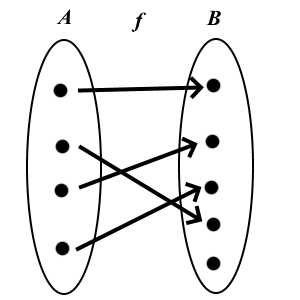 is one-to-one but not onto
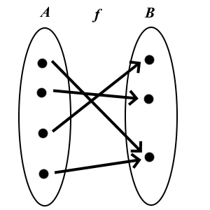 is onto but not one-to-one
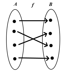 is one-to-one and onto
Transcendental functions
Trigonometric functions
Unit of measurement of an angle = rad: the arclength of the arc on the unit circle, that corresponds to the angle.
 rad =
rad =  degrees, i.e. rad =
  degrees
The functions
 are defined in terms of the unit circle so that
") ,
, ![x\in [0,2\pi]](https://mycourses.aalto.fi/filter/tex/pix.php/45279ec769d88b24314782eea30c7f1e.gif "x\in [0,2\pi]") , is the point on the unit circle corresponding to the
angle , measured counterclockwise from the point
, is the point on the unit circle corresponding to the
angle , measured counterclockwise from the point ") .
.
,")
")
Periodicity:
 = \sin x,\ \cos (x+2\pi)=\cos x,")
 = \tan x")
 ,
, =1")
 ,
, = 0")
Parity:
and are odd functions, is an even function:
 = -\sin x,")
 = \cos x,")
 = -\tan x.")
 for all
 Proof: Pythagorean Theorem.
Addition formulas:
 = \sin x \cos y +\cos x \sin y")
 = \cos x \cos y -\sin x \sin y")
Basic properties (from the unit circle!)
Proof: Geometrically, or more easily with vectors and matrices.
Derivatives:
 = \cos x,\ \ D(\cos x) = -\sin x")
Example
It follows that the functions
=\sin (\omega t)") and
and =\cos (\omega t)") satisfy the
differential equation
satisfy the
differential equation
+\omega^2y(t)=0,") that models harmonic oscillation. Here is the time variable
and the constant
that models harmonic oscillation. Here is the time variable
and the constant  is the angular frequency of the oscillation.
We will see later that all the solutions of this differential equation
are of the form
is the angular frequency of the oscillation.
We will see later that all the solutions of this differential equation
are of the form
=A\cos (\omega t) +B\sin (\omega t),") with
with  constants. They will be uniquely determined if we know
the initial location
constants. They will be uniquely determined if we know
the initial location ") and the initial velocity
and the initial velocity ") . All solutions
are periodic and their period is
. All solutions
are periodic and their period is  .
.
 = y_{0}\cos(\omega t)") ,
,where
is the elapsed time in secondsArcus functions
The trigonometric functions have inverses if their domain and codomains are chosen in a suitable way.
The Sine function
![\sin \colon [-\pi/2,\pi/2]\to [-1,1]](https://mycourses.aalto.fi/filter/tex/pix.php/8516ac159a27828b8807ae8346208684.gif "\sin \colon [-\pi/2,\pi/2]\to [-1,1]") is strictly increasing and bijective.
is strictly increasing and bijective.The Cosine function
![\cos \colon [0,\pi] \to [-1,1]](https://mycourses.aalto.fi/filter/tex/pix.php/7b6724fb6d58f64ba500defadc44773d.gif "\cos \colon [0,\pi] \to [-1,1]") is strictly decreasing and bijective.
is strictly decreasing and bijective.The tangent function
![\tan \colon ]-\pi/2,\pi/2[\, \to \mathbb{R}](https://mycourses.aalto.fi/filter/tex/pix.php/04f0656b3b1805879518b5a4d600ae97.gif "\tan \colon ]-\pi/2,\pi/2[\, \to \mathbb{R}") is strictly increasing and bijective.
is strictly increasing and bijective.
Arcus functions
Inverses:
![\arctan \colon \mathbb{R}\to \ ]-\pi/2,\pi/2[,](https://mycourses.aalto.fi/filter/tex/pix.php/5a0cfc94ec76b4bb98759ea997a6814e.gif "\arctan \colon \mathbb{R}\to \ ]-\pi/2,\pi/2[,")
![\arcsin \colon [-1,1]\to [-\pi/2,\pi/2],](https://mycourses.aalto.fi/filter/tex/pix.php/c4d09554c2fd5fc1cbf2d81a599c1b95.gif "\arcsin \colon [-1,1]\to [-\pi/2,\pi/2],")
![\arccos \colon [-1,1]\to [0,\pi]](https://mycourses.aalto.fi/filter/tex/pix.php/ae1f9e9c619a7daceef40e2227521839.gif "\arccos \colon [-1,1]\to [0,\pi]")
This means:
![x = \tan \alpha \Leftrightarrow \alpha = \arctan x \ \ \text{for } \alpha \in \ ]-\pi/2,\pi/2[](https://mycourses.aalto.fi/filter/tex/pix.php/1e8adfc9de7373123d3e37d24295583b.gif "x = \tan \alpha \Leftrightarrow \alpha = \arctan x \ \ \text{for } \alpha \in \ ]-\pi/2,\pi/2[")
![x = \sin \alpha \Leftrightarrow \alpha = \arcsin x \ \ \text{for } \alpha \in \, [-\pi/2,\pi/2]](https://mycourses.aalto.fi/filter/tex/pix.php/e0f134a17e198c541c553b3c2e9305f0.gif "x = \sin \alpha \Leftrightarrow \alpha = \arcsin x \ \ \text{for } \alpha \in \, [-\pi/2,\pi/2]")
![x = \cos \alpha \Leftrightarrow \alpha = \arccos x \ \ \text{for } \alpha \in \, [0,\pi]](https://mycourses.aalto.fi/filter/tex/pix.php/eab3cb1a5193c48cde03e2046ec37027.gif "x = \cos \alpha \Leftrightarrow \alpha = \arccos x \ \ \text{for } \alpha \in \, [0,\pi]")
The graphs of and  .
.
Derivatives of the arcus functions


Note. The first result is very useful in integration.
Here we will only prove the first result (1). By differentiating
both sides of the equation =x") for :
for :
\bigr) \cdot D(\arctan x) = D x = 1")
= \frac{1}{1+\tan^2(\arctan x)}")

The last row follows also directly from the formula for the derivative of an inverse.
Example
Show that
 for
for  .
.
Example
Derive the addition formula for tan, and show that

Solutions: Voluntary exercises. The first can be deduced by looking at
a rectangular triangle with the length of the hypotenuse equal to 1
and one leg of length .
Introduction: Radioactive decay
Let ") model the number of radioactive nuclei at time .
During a short time interval
model the number of radioactive nuclei at time .
During a short time interval  the number of decaying nuclei is (approximately) directly proportional to
the length of the interval, and also to the number of nuclei at time :
the number of decaying nuclei is (approximately) directly proportional to
the length of the interval, and also to the number of nuclei at time :
-y(t) \approx -k\cdot y(t)\cdot \Delta t.") The constant depends on the substance and is called the decay constant.
From this we obtain
The constant depends on the substance and is called the decay constant.
From this we obtain
,") and in the limit as
and in the limit as  we end up with the differential equation
 =-ky(t)") .
.
Exponential function
Definition: Euler's number
Euler's number (or Napier's constant) is defined as
 ^n = 1+1+\frac{1}{2!}+\frac{1}{3!} +\frac{1}{4!}
+\dots")

Definition: Exponential function
The Exponential function exp:
 = \sum_{k=0}^{\infty} \frac{x^k}{k!}=
\lim_{n\to \infty} \left( 1+\frac{x}{n}\right) ^n = e^x.") This definition (using the series expansion) is based on the conditions
This definition (using the series expansion) is based on the conditions
=\exp(x)") and
and =1") , which imply
that
, which imply
that }(0)=\exp(0)= 1") for all ,
so the Maclaurin series is the one above.
for all ,
so the Maclaurin series is the one above.
The connections between different expressions are surprisingly tedious to prove, and we omit the details here. The main steps include the following:
Define
 ,
,
 =\sum_{k=0}^{\infty}\frac{x^k}{k!}.") This series converges for all (ratio test).
This series converges for all (ratio test).Show: exp is differentiable and satisfies
for all . (This is the most difficult part but intutively rather
obvious, because in practice we just differentiate the series
term by term like a polynomial.)
It has the following properties =1") ,
,
=1/\exp (x) \text{ and }
\exp (x+y)=\exp (x)\, \exp(y)") for all
for all  .
.
These imply that =(\exp (1))^{p/q}") for all rational numbers
for all rational numbers  .
.
By continuity
 =(\exp (1))^x") for all .
for all .
Since
 = \sum_{k=0}^{\infty}\frac{1}{k!}
=\lim_{n\to \infty} \left( 1+\frac{1}{n}\right) ^n=e,") we obtain the form
we obtain the form  .
.
?
Corollary
It follows from above that ![\exp\colon\mathbb{R}\to\, ]0,\infty[](https://mycourses.aalto.fi/filter/tex/pix.php/463736f26c065deb116e8539cc1e1c90.gif "\exp\colon\mathbb{R}\to\, ]0,\infty[") is strictly increasing,
bicective, and
is strictly increasing,
bicective, and
 = \infty,\
\lim_{x\to-\infty}\exp(x) = 0,\
\lim_{x\to\infty}\frac{x^n}{\exp (x)} = 0 \text{ for all } n\in \mathbf{N}.")
From here on we write ") . Properties:
. Properties:


 = e^x")

^y = e^{xy}") .
.
Differential equation 
Theorem
Let  be a constant. All solutions
 ") of the ordinary differenial equation (ODE)
of the ordinary differenial equation (ODE)
=ky(x),\ x\in \mathbb{R},") are of the form
are of the form =Ce^{kx}") , where
, where  is a constant. If we know
the value of at some point , then the constant
is a constant. If we know
the value of at some point , then the constant
 will be uniquely determined.
Suppose that =ky(x)") . Then
. Then
e^{-kx})= y'(x)e^{-kx}+y(x)\cdot (-ke^{-kx})")
e^{-kx}-ky(x)e^{-kx}=0") for all
for all  , so that
 e^{-kx}=C=") constant.
Multiplying both sides with
constant.
Multiplying both sides with  we obtain .
Euler's formula
Definition: Complex numbers
Imaginary unit  : a strange creature satisfying
  . The complex numbers
are of the form
. The complex numbers
are of the form  , where . We will return to these later.
Theorem: Euler's formula
If we substitute  as a variable in the expontential fuction, and
collect real terms separately, we obtain Euler's formula
as a variable in the expontential fuction, and
collect real terms separately, we obtain Euler's formula

 in the definition of the exponential function and write the series as the sum
of its even (
in the definition of the exponential function and write the series as the sum
of its even ( ) and odd
 ") parts. Note that
parts. Note that ^k = (-1)^{k}") and remember the Taylor series of the trigonometric
functions.
and remember the Taylor series of the trigonometric
functions.
As a special case we have Euler's identity  .
It connects the most important numbers , , ,
.
It connects the most important numbers , , ,  ja and the
three basic operations sum, multiplication, and power.
ja and the
three basic operations sum, multiplication, and power.
Using  we can also derive the
expressions
we can also derive the
expressions
,\
\sin x=\frac{1}{2i}\bigl( e^{ix}-e^{-ix}\bigr),
\ x\in\mathbb{R}.")
") and the partial sums
and the partial sums 
Logarithms
Definition: Natural logarithm
Natural logarithm is the inverse of the exponential function:
![\ln\colon \ ]0,\infty[ \ \to \mathbb{R}](https://mycourses.aalto.fi/filter/tex/pix.php/a57877163d9051a40ddff6a55fb8ea50.gif "\ln\colon \ ]0,\infty[ \ \to \mathbb{R}")
Note. The general logarithm with base is based on the
condition
 for
for  and
and  .
.
Beside the natural logarithm, in applications also appear the
Briggs logarithm with base 10:  , and the binary
logarithm with base 2:
, and the binary
logarithm with base 2:  .
.
Usually (e.g. in mathematical software)  is the same as
 .
.
Properties of the logarithm:
 for
for  =x") for
for  ,
, 
 = b\ln a") if ,
if ,  = \ln a+\ln b") , if
, if 
 for
for 
These follow from the corresponding properties of exp.
Example
Substituting  and
and  to the formula
 we obtain
 = \ln a +\ln b") .
.

Hyperbolic functions
Definition: Hyperbolic functions
Hyperbolic sine sinus hyperbolicus  ,
hyperbolic cosine cosinus hyperbolicus
,
hyperbolic cosine cosinus hyperbolicus  and hyperbolic tangent
 are defined as
")
")
![\tanh \colon \mathbb{R}\to \ ]-1,1[, \ \tanh x =\frac{\sinh x}{\cosh x}](https://mycourses.aalto.fi/filter/tex/pix.php/2ac4198587d98a4f7dd3df05218f66f7.gif "\tanh \colon \mathbb{R}\to \ ]-1,1[, \ \tanh x =\frac{\sinh x}{\cosh x}")
Properties:  ; all trigonometric have their hyperbolic counterparts,
which follow from the properties
; all trigonometric have their hyperbolic counterparts,
which follow from the properties =i\sin x") ,
, =\cos x") .
In these formulas, the sign of
.
In these formulas, the sign of  will change, but the other signs remain the same.
Derivatives:  ,
,  .
.
Hyperbolic inverse functions: the so-called area functions;
area and the shortening ar refer to a certain geometrical area
related to the hyperbola  :
:
 ,\ x\in\mathbb{R}")
 ,\ x\ge 1")
Derivatives of the inverse functions:


',
radius : .4,
label : { useMathJax : true, strokeColor : 'black', offset : [0, .5] }
});
var info = board.create('text', [-1.2, -1.25, function() {
return '=(' + Math.cos(x.Value()).toFixed(3) + ',' + Math.sin(x.Value()).toFixed(3) + ')") ';
}], {
useMathJax : true,
fixed : true
});
board.fullUpdate();
})();
';
}], {
useMathJax : true,
fixed : true
});
board.fullUpdate();
})();
7. Area
Table of Content
Area in the plane
We consider areas of plane sets bounded by closed curves. In the more general cases, the concept of area becomes theoretically very difficult.
The area of a planar set is defined by reducing to the areas of simpler sets. The area cannot be "calculated", unless we first have a definition of "area" (although this is common practice in school mathematics).
Starting point
The area of a rectangle
The area of a rectangle is

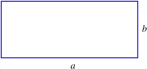
Definition: Area of a Parallelogram
The area of a parallelogram is 
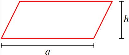
Definition: Area of a triangle
The area of a triangle is (by definition)

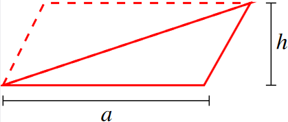
Polygon
A (simple) polygon is a plane set bounded by a closed curve that consists of a finite number of line segments without self-intersections.
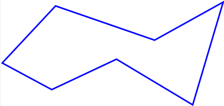
Definition: Area of a polygon
The area of a polygon is defined by dividing it into a
finite number of triangles (called a
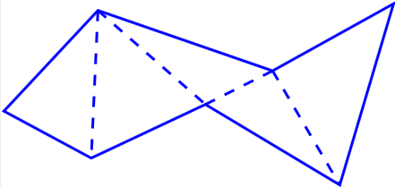
Theorem.
The sum of the areas of triangles in a triangulation of a polygon is the same for all triangulations.
General case
For a plane set  bounded by a closed curve we can construct
inner polygons
bounded by a closed curve we can construct
inner polygons  and outer polygons
 :
:  .
.
 has an area if for every
  there is an inner polygon
  and an outer polygon , whose areas differ by less
than :
and an outer polygon , whose areas differ by less
than :
-A(P_i)") This implies that between all areas
This implies that between all areas ") and
and ") there is a unique real number
there is a unique real number ") ,
which is (by definition) the area of .
,
which is (by definition) the area of .
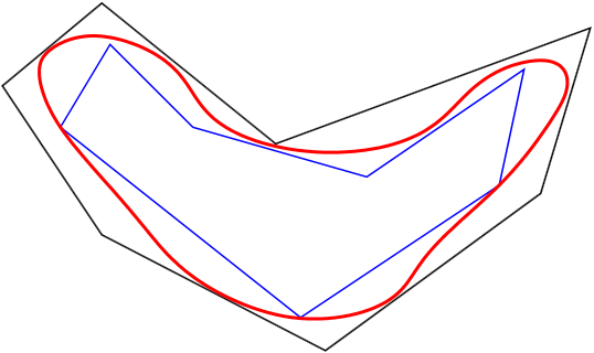
A surprise: The condition that is bounded by a closed curve (without self-intersections)
does not guarantee that it has an area! Reason: The boundary curve can be so "wiggly",
that it has positive "area". The first such example was constucted by [W.F. Osgood, 1903]:
Example
Derive the formula  for a circle with radius by choosing
regular inscrided and circumscribed -gons as inner and outer polygons,
and let .
for a circle with radius by choosing
regular inscrided and circumscribed -gons as inner and outer polygons,
and let .
The solution is a voluntary exercise, where you need the limit
 Hint: Show that the inscribed and circumscribed areas are
}{2\pi/n} \ \text{ and }\ \pi R^2\frac{\tan \pi/n}{\pi/n}.")
8. Integral
From sum to integral
Definite integral
Geometric interpretation: Let ![f\colon[a,b]\to\mathbb{R}](https://mycourses.aalto.fi/filter/tex/pix.php/4bbb5ba4231dc6733dfafd89107596a5.gif "f\colon[a,b]\to\mathbb{R}") be such that
be such that \ge 0") for all
for all
![x\in[a,b]](https://mycourses.aalto.fi/filter/tex/pix.php/c7c42309c359c25dfe77f397d5261997.gif "x\in[a,b]") . How can we find the area of the region bounded by the function graph , the
x-axis and the two lines
. How can we find the area of the region bounded by the function graph , the
x-axis and the two lines  and
and  ?
?
The answer to this question is given by the definite integral
\,dx") Remark. The general definition of the integral does not necessitate the condition .
Remark. The general definition of the integral does not necessitate the condition .
Integration of continuous functions
Definition: Partition
Let be continuous. A finite sequence ") of real numbers such that
of real numbers such that
 is called a partition of the interval .
from to Definition: Upper and lower sum
For each partition we define the related upper sum of the function as
 = \sum_{k=1}^{n}M_{k}(x_{k}-x_{k-1}),~M_{k} = \max\{f(x)\mid x_{k-1}\le x\le x_{k}\}") and the lower sum as
and the lower sum as
 = \sum_{k=1}^{n}m_{k}(x_{k}-x_{k-1}),~m_{k}=\min\{f(x)\mid x_{k-1}\le x\le x_{k}\}.")
If is a positive function then the upper sum represents the total area of the rectangles circumscribing
the function graph and similarly the lower sum is the total area of the inscribed rectangles.
Properties of partitions
- Suppose that
 and
and  are two partitions of a given interval such that is a subsequence of
(i.e. is finer than ). Then the inequalities
are two partitions of a given interval such that is a subsequence of
(i.e. is finer than ). Then the inequalities
always hold. \ge U_{D_{2}}(f)~") and
and  \le L_{D_{2}}(f)")
- For any two partitions and of a given interval the inequality
 \le U_{D_{1}}(f)") always holds.
always holds.
=~")
| Upper Darboux sum | Lower Darboux sum |
Definition: Integrability
We say that a function is integrable if for every  there exists a corresponding partition of such that
 - L_{D}(f) < \epsilon.")
Definition: Integral
Integrability implies that there exists a unique real number such that \le I\le U_{D}(f)") for every
partition . This is called the integral of over the interval and denoted by
for every
partition . This is called the integral of over the interval and denoted by
\,dx.")
Remark. This definition of the integral is sometimes referred to as the Darboux integral.
For non-negative functions this definition of the integral coincides with the idea of making the difference
between the the areas of the circumscribed and the inscribed rectangles arbitrarily small by using ever finer partitions.
Theorem.
A continuous function on a closed interval is integrable.
Here we will only provide the proof for continuous functions with bounded derivatives.
Suppose that is a continuous function and that there exists a constant  such that
|\le L") for all
for all ![x\in]a,b[](https://mycourses.aalto.fi/filter/tex/pix.php/446e008dffdc84c23608a41270477f2f.gif "x\in]a,b[") . Let and define to be an equally spaced partition of such that
. Let and define to be an equally spaced partition of such that
},~\text{for all} k=1,2,\dots,n.") Let
Let =m_{k}") and
and =M_{k}") for some suitable points
for some suitable points ![y_{k},z_{k}\in[x_{k-1},x_{k}]](https://mycourses.aalto.fi/filter/tex/pix.php/b0cc09fba8e4e83e7252a84f0c0d25e5.gif "y_{k},z_{k}\in[x_{k-1},x_{k}]") . The mean value theorem
then states that
. The mean value theorem
then states that
|z_{k}-y_{k}|\le L\Delta x") and thus
and thus
-L_{D}(f) = \sum_{k=1}^{n}(M_{k}-m_{k})\Delta x < \frac{\epsilon}{b-a}\sum_{k=1}^{n}\Delta x = \epsilon.")
Definition: Riemann integral
Suppose that is a continuous function and let
") be a partition of
be a partition of ![\left[a,b\right]](https://mycourses.aalto.fi/filter/tex/pix.php/22be842f9527b4b0ef3b7085b5486b7b.gif "\left[a,b\right]") and
and
") be a sequence of real numbers such that
be a sequence of real numbers such that
![z_{k}\in[x_{k-1},x_{k}]](https://mycourses.aalto.fi/filter/tex/pix.php/6699d41c4ee1c2de849bc6a2162fd4e7.gif "z_{k}\in[x_{k-1},x_{k}]") for all
for all  . The partial sums
\Delta x_{k},~\text{where}
~\Delta x_{k}=x_{k}-x_{k-1}") are called the Riemann sums of . Suppose further that the partitions are
such that
are called the Riemann sums of . Suppose further that the partitions are
such that  as .
The integral of can then be defined as the limit
as .
The integral of can then be defined as the limit
\,\mathrm{d}x = \lim_{n\to\infty} S_{n}.") This definition of the integral is called the Riemann integral.
This definition of the integral is called the Riemann integral.
Remark. This definition of the integral turns out to be equivalent to that of the Darboux integral i.e. a function is Riemann-integrable if and only if it is Darboux-integrable and the values of the two integrals are always equal.
Example
Find the integral of =x") over the interval
over the interval ![[0,1]](https://mycourses.aalto.fi/filter/tex/pix.php/ccfcd347d0bf65dc77afe01a3306a96b.gif "[0,1]") using Riemann sums.
using Riemann sums.
Let  . Then
  ,
,  and
and  for all
 . Thus the sequence
 ") is a proper
partition of
is a proper
partition of ![\left[0,1\right]](https://mycourses.aalto.fi/filter/tex/pix.php/4f27db35c23e1b587a92f6ba055a4b94.gif "\left[0,1\right]") . This partition has the pleasant property hat
. This partition has the pleasant property hat
 is a constant. Estimating the Riemann sums we now find that
\Delta x = \sum_{k=1}^{n}x_{k}\Delta x=
\sum_{k=1}^{n}\frac{k}{n}\left(\frac{1}{n}\right)")
}{2} = \frac{n+1}{2n}\to
\frac{1}{2},") as and hence
as and hence
\,\mathrm{d}x = \frac{1}{2}.")
This is of course the area of the triangular region bounded by the line ,
the -axis and the lines and .
Remark. Any interval can be partitioned into equally spaced subintervals by setting
/n") and
and  .
.
Conventions
- If the upper and lower limits of integration are the same then the integral is zero:
\,dx = 0.")
- Reversing the limits of integration changes the sign of the integral:
\,dx = -\int_{a}^{b}f(x)\,dx.")
- It also follows that
\,dx = \int_{a}^{c}f(x)\,dx + \int_{c}^{b}f(x)\,dx") holds for all
holds for all  .
.
Piecewise-defined functions
Definition: Piecewise continuity
A function ![f\colon\left[a,b\right]\to\mathbb{R}](https://mycourses.aalto.fi/filter/tex/pix.php/651a926e83a81b2331659e5bec837922.gif "f\colon\left[a,b\right]\to\mathbb{R}") is called piecewise continuous
if it is continuous except at a finite number of points
is called piecewise continuous
if it is continuous except at a finite number of points
 and the one-sided limits of the function are defined and bounded on each of these
points. It follows that the restriction of on each subinterval
and the one-sided limits of the function are defined and bounded on each of these
points. It follows that the restriction of on each subinterval
![\left[c_{k-1},c_{k}\right]](https://mycourses.aalto.fi/filter/tex/pix.php/4c8251634c3e4dcef42dea1404161757.gif "\left[c_{k-1},c_{k}\right]") is continuous if the one-sided limits are taken to
be the values of the function at the end points of the subinterval.
is continuous if the one-sided limits are taken to
be the values of the function at the end points of the subinterval.
Definition: Piecewise integration
Let ![f\colon\left[a,b\right]](https://mycourses.aalto.fi/filter/tex/pix.php/9f37a3c940314dccb310e7db856fb524.gif "f\colon\left[a,b\right]") be a piecewise continuous function. Then
be a piecewise continuous function. Then
\,dx = \sum_{k=1}^{m+1}\int_{c_{k-1}}^{c_{k}}f(x)\,dx,") where
where  and is thought as a
continuous function on each subinterval . Usually
functions which are continuous yet piecewise defined are also integrated using the
same idea.
and is thought as a
continuous function on each subinterval . Usually
functions which are continuous yet piecewise defined are also integrated using the
same idea.
Example
Consider the function ![f\colon\left[-1,1\right]](https://mycourses.aalto.fi/filter/tex/pix.php/8fa1143ca458419d8b2c9fe6b3bc7b98.gif "f\colon\left[-1,1\right]") defined as
defined as
 =
\begin{cases}
-1 &\text{ for }-1\le x") We can now integrate as follows:
We can now integrate as follows:
\,dx = \int_{-1}^{0}f(x)\,dx + \int_{0}^{1}f(x)\,dx")
\,dx + \int_{0}^{1}1\,dx = -1\cdot(-1-0) + 1\cdot(1-0) = 2.")
 =\begin{cases}
-1 &\text{ for }-1\le x")
Important properties
Properties
Suppose that ![f,g\colon\left[a,b\right]\to\mathbb{R}](https://mycourses.aalto.fi/filter/tex/pix.php/f01d397fa4a741a5373783b544f03897.gif "f,g\colon\left[a,b\right]\to\mathbb{R}") are piecewise continuous
functions. The integral has the following properties
are piecewise continuous
functions. The integral has the following properties
- Linearity: If
 then
then
+c_{2}g(x)\big)\,\mathrm{d}x = c_{1}\int_{a}^{b}f(x)\,\mathrm{d}x+c_{2}\int_{a}^{b}g(x)\,\mathrm{d}x.")
- If
\ge 0") for all then
for all then
\,\mathrm{d}x \ge 0.")
- If
\le g(x)") then
then
\,\mathrm{d}x \le \int_{a}^{b}g(x)\,\mathrm{d}x.")
- As
\le|f(x)|") it follows that
it follows that
\,\mathrm{d}x \le \int_{a}^{b}|f(x)|\,\mathrm{d}x") and taking the absolute value of both sides of the equation gives
and taking the absolute value of both sides of the equation gives
\,\mathrm{d}x\right|\le \int_{a}^{b}|f(x)|\,\mathrm{d}x.")
- Suppose that
![p=\inf_{x\in\left[a,b\right]}f(x)](https://mycourses.aalto.fi/filter/tex/pix.php/df0ba13db5d97e1ab617c25bf3f053f3.gif "p=\inf_{x\in\left[a,b\right]}f(x)") and
and ![s=\sup_{x\in\left[a,b\right]}f(x)](https://mycourses.aalto.fi/filter/tex/pix.php/74dbac954365a4026b75091df793c18d.gif "s=\sup_{x\in\left[a,b\right]}f(x)") . Then
. Then
\le \int_{a}^{b}f(x)\,dx \le s(b-a).")
Fundamental theorem of calculus
Theorem: Mean value theorem
Let be a continuous function. Then there exists such that
=\frac{1}{b-a}\int_{a}^{b}f(x)\,\mathrm{d}x.") This is the mean value of on the interval and we denote it with
This is the mean value of on the interval and we denote it with  .
.
Suppose that  and are the minimum and maximum of on the interval , respectively. It follows that
\le \int_{a}^{b}f(x)\,\mathrm{d}x\le M(b-a)") or
or
\,\mathrm{d}x\le M\quad \Leftrightarrow\quad m\le \overline{f}\le M.") Thus is between the minimum and maximum of a continuous function and by the intermediate value theorem
it must be that
Thus is between the minimum and maximum of a continuous function and by the intermediate value theorem
it must be that =\overline{f}") for some
for some ![c\in\,]a,b[](https://mycourses.aalto.fi/filter/tex/pix.php/0645c1a33227f3466be2997827a643b5.gif "c\in\,]a,b[") .
.
(First) Fundamental theorem of calculus.
Let be a continuous function. Then
\,\mathrm{d}t = f(x)") for all
for all ![x\in\,]a,b[](https://mycourses.aalto.fi/filter/tex/pix.php/72fa533e00aaedd77d6d52d82313b48e.gif "x\in\,]a,b[") .
.
Let
 = \int_{a}^{x}f(t)\,\mathrm{d}t.") The mean value theorem implies that there exists
The mean value theorem implies that there exists ![c\in\,[x,x+h]](https://mycourses.aalto.fi/filter/tex/pix.php/318888fc5bb357cd31a47f39bdaf0103.gif "c\in\,[x,x+h]") such that
such that
-F(x)}{h} = \frac{1}{h}\left(\int_{a}^{x+h}f(t)\,
\mathrm{d}t-\int_{a}^{x}f(t)\,\mathrm{d}t\right)")
\,\mathrm{d}t = \frac{1}{h}f(c)(x+h-x) = f(c).") As
As  we see that
  and from the continuity of it follows that
\to f(x)") . Thus
. Thus =f(x)") .
.
Antiderivative
If on some open interval then  is the antiderivative
(or the primitive function) of . The fundamental theorem of calculus
guarantees that for every continuous function there exists an antiderivative
is the antiderivative
(or the primitive function) of . The fundamental theorem of calculus
guarantees that for every continuous function there exists an antiderivative
 = \int_{a}^{x}f(t)\,dt.") The antiderivative is not necessarily expressible as a combination of elementary
functions even if were an elementary function, e.g.
The antiderivative is not necessarily expressible as a combination of elementary
functions even if were an elementary function, e.g.  = e^{-x^{2}}") .
Such primitives are called nonelementary antiderivatives.
.
Such primitives are called nonelementary antiderivatives.
Theorem.
Antiderivatives are only unique up to a constant;
\,dx = F(x) + C, C\in\mathbb{R} \text{ constant }") if .
if .
Suppose that =F'_{2}(x)=f(x)") for all . Then the derivative of
for all . Then the derivative of -F_{2}(x)") is identically zero and thus the difference is a constant.
is identically zero and thus the difference is a constant.
(Second) Fundamental theorem of calculus
Let be a continuous function and  an antiderivative of , then
\,dx = G(x)\Big|_{x=a}^{x=b} = G(b)-G(a).")
Because =\int_{a}^{x}f(t)\,dt") is an antiderivative of then due to continuity
is an antiderivative of then due to continuity -G(x)=C=\text{constant}") for all
for all ![x\in\left[a,b\right]](https://mycourses.aalto.fi/filter/tex/pix.php/2f48f5b87131a8927f62cdab351ef9f5.gif "x\in\left[a,b\right]") . Substituting we find that
. Substituting we find that ") . Thus
. Thus
\,dt = F(x) = G(x)-G(a)") and substituting the result follows.
and substituting the result follows.
Suppose that is a continuous function and that and are
differentiable functions. Then
}^{b(x)}f(t)\,dt = f(b(x))b'(x)-f(a(x))a'(x).")
Suppose that is an antiderivative of . Then from the fundamental theorem of calculus and the chain rule it follows that
}^{b(x)}f(t)\,dt = \frac{d}{dx}\big(F(b(x)) - F(a(x))\big)")
) - \frac{d}{dx}F(a(x)) = F'(b(x))b'(x) - F'(a(x))a'(x)")
)b'(x) - f(a(x))a'(x).")
Integrals of elementary functions
Constant Functions
Given the constant function  = c,\,c\in\mathbb{R}") . The integral
. The integral \,\mathrm{d} x = \int\limits_a^b c \, \mathrm{d}x") has to be determined now.
has to be determined now.
Solution by finding a antiderivative
From the previous chapter it is known that  = c\cdot x") gives
gives  = c") . This means that
. This means that  is an antiderivative for . So the following applies
 ![\int\limits_a^b c \, \mathrm{d}x = [c \cdot x]_{x=a}^{x=b} = c\cdot b - c \cdot a = c \cdot (b-a).](https://mycourses.aalto.fi/filter/tex/pix.php/8665eaa9c4f246caaa2ed563cb0a03e8.gif "\int\limits_a^b c \, \mathrm{d}x = [c \cdot x]_{x=a}^{x=b} = c\cdot b - c \cdot a = c \cdot (b-a).")
Remark: Of course, a function  = c \cdot x + d") would also be an antiderivative of , since the constant is omitted in the derivation. For sake of simplicity can be used, since can be chosen as
would also be an antiderivative of , since the constant is omitted in the derivation. For sake of simplicity can be used, since can be chosen as  for definite integrals.
Solution by geometry
The area under the constant function forms a rectangle with height and length  . Thus the area is
 ") and this corresponds to the solution of the integral. Illustrate this remark by a sketch.
and this corresponds to the solution of the integral. Illustrate this remark by a sketch.
Linear functions
Given is the linear function  = mx") . We are looking for the integral
. We are looking for the integral \, \mathrm dx=\int\limits_a^b mx\, \mathrm dx") .
.
Solve by finding a antiderivative
The antiderivative of a linear function is in any case a quadratic function, since  . The derivative of a quadratic function results in a linear function. Here, it is important to consider the leading factor as in
 }{\mathrm dx} = mx.") Thus the result is
Thus the result is ![\int\limits_a^b mx \mathrm{d}x = \left[\frac{m}{2}x^2 \right]_{x=a}^{x=b}= \frac{m}{2}b^2 - \frac{m}{2}a^2.](https://mycourses.aalto.fi/filter/tex/pix.php/b5241a45e0cf510936549697bfb8ec04.gif "\int\limits_a^b mx \mathrm{d}x = \left[\frac{m}{2}x^2 \right]_{x=a}^{x=b}= \frac{m}{2}b^2 - \frac{m}{2}a^2.")
Solving by geometry
The integral  can be seen geometrically, as subtracting the triangle with the edges
 ") ,
, ") and
and ") from the triangle with the edges ,
from the triangle with the edges , ") and
and ") . Since the area of a triangle ist given by
. Since the area of a triangle ist given by  , the area of the first triangle
  and that of the second triangle is analogous
  . For the integral the result is
  . This is consistent with the integral calculated using the antiderivative. Illustrate this remark by a sketch.
Power functions
In constant and linear functions we have already seen that the exponent of a function decreases by one when it is derived. So it has to get bigger when integrating.
The following applies:  It follows that the antiderivative for
  must have the exponent
  ,
,  \cdot x^n.") By multiplying the last equation with
By multiplying the last equation with  we get
  Finally the antiderivative is
  .
.
Examples


The formula ![\int x^n\, \mathrm dx = [\frac{1}{n+1} x^{n+1}]](https://mycourses.aalto.fi/filter/tex/pix.php/222a5eca783899397010e410d9be1ac6.gif "\int x^n\, \mathrm dx = [\frac{1}{n+1} x^{n+1}]") is also valid, if the exponent of the function is a real number and not equal
is also valid, if the exponent of the function is a real number and not equal  .
.
Examples


- But: For
 applies
+c,\,c\in\mathbb{R}.")
Natural Exponential function
The natural exponential function  = e^x") is one of the easiest function to differentiate and integrate.
Since the derivation of results in , it follows
is one of the easiest function to differentiate and integrate.
Since the derivation of results in , it follows 
Example 1
Determine the value of the integral  .
.

Example 2
Determine the value of the integral  . Using the same considerations as above we get
 =\frac{1}{\alpha}\left(e^{\alpha b}-1\right).") Important is here, that we have to use the factor
Important is here, that we have to use the factor  .
.
Natural Logarithm
The derivative of the natural logarithmic function is  =\frac{1}{x}") for . It even applies to . These results together result in for the antiderivative of
for . It even applies to . These results together result in for the antiderivative of 
 +c , c\in\mathbb{R}.")
An antiderivative can be specified for the natural logarithm: \,\mathrm{d}x = x\ln(x) - x + c ,\, c\in\mathbb{R}.")
Trigonometric function
The antiderivatives of and also result logically if you derive "backwards". We have
\, \mathrm dx = -\cos(x)+c,\,c\in\mathbb{R},") since
since )' =-(-\sin(x))=\sin(x).") Furthermore we know
Furthermore we know \, \mathrm dx = \sin(x)+c,\,c\in\mathbb{R},") since
since )' = \cos(x)") applies.
applies.
Example 1
Which area is covered by the sine on the interval ![[0,\pi]](https://mycourses.aalto.fi/filter/tex/pix.php/a79560c6f70853be01bb23f7539e168c.gif "[0,\pi]") and the -axis?
To determination the area we simply have to evaluate the integral
and the -axis?
To determination the area we simply have to evaluate the integral
 \, \mathrm{\tau}.") That means
That means ![\int_0^{\pi} \sin(\tau) \, \mathrm{d}\tau = \left[-\cos(\tau)\right]_{\tau=0}^{\tau=\pi} =
-\cos(\pi) - (-\cos(0)) = -(-1) - (-1) = 2.](https://mycourses.aalto.fi/filter/tex/pix.php/ed010b1da078996da59e937f6091bf5f.gif "\int_0^{\pi} \sin(\tau) \, \mathrm{d}\tau = \left[-\cos(\tau)\right]_{\tau=0}^{\tau=\pi} =
-\cos(\pi) - (-\cos(0)) = -(-1) - (-1) = 2.") Again make a sketch for this example.
Again make a sketch for this example.
Example 2
How can the integral \,\mathrm{d}t") be expressed analytically?
be expressed analytically?
To determine the integral we use the antiderivative of the cosine:  = \cos(x)") . However, the inner derivativ has to be considered in the
given function and thus we get
. However, the inner derivativ has to be considered in the
given function and thus we get \,\mathrm{d}t =\frac{1}{\omega}\sin(\omega t+\phi)+c,\,c\in\mathbb{R}.")
Summary:
The most common antiderivatives follow from the rules of differentiation:


Example 1
Evaluate the integrals  and
and \,dx") .
.
Solution. The antiderivative of  is
is  so we have that
 The antiderivative of
 ") is
is ") and thus
and thus
\,dx = -\frac{1}{\pi}(\cos\pi-\cos0) = \frac{2}{\pi}.")
Example 2
Evaluate the integral  .
.
Solution. The antiderivative might look something like =a(25-9x^{2})^{1/2}") , where we can find the factor through differentiation:
, where we can find the factor through differentiation:
^{1/2}\big) = a\cdot\frac{1}{2}\cdot(-18x)(25-9x^{2})^{-1/2} = \frac{-9ax}{\sqrt{25-9x^{2}}}") hence if
hence if  we get the correct antiderivative. Thus
^{1/2}\Big|_{x=0}^{x=1} = -\frac{1}{9}(\sqrt{16}-\sqrt{25}) = \frac{1}{9}.") This integral can also be solved using integration by substitution; more on this method later.
This integral can also be solved using integration by substitution; more on this method later.
Geometric applications
Area of a plane region
Suppose that and are piecewise continuous functions. The area of a region bounded by the graphs , and the vertical lines and is given by the integral
-g(x)|\,dx.")
Especially if is a non-negative function on the interval and =0") for all then the integral
for all then the integral
\,dx") is the area of the region bounded by the graph , the -axis and the vertical lines and .
is the area of the region bounded by the graph , the -axis and the vertical lines and .
Arc length
The arc length  of a planar curve between points and is given by the integral
^{2}}\,dx.")
Heuristic reasoning: On a small interval ![\left[x,x+\Delta x\right]](https://mycourses.aalto.fi/filter/tex/pix.php/4d8fd407309f8f47e5b678de4fddac7f.gif "\left[x,x+\Delta x\right]") the arc length of the curve between and
the arc length of the curve between and ") is approximately
is approximately
^{2}} \approx \Delta x\sqrt{1+f'(x)^{2}}.")
 .
.Surface of revolution
The area of a surface generated by rotating the graph around the -axis on the interval is given by
|\sqrt{1+f'(x)^{2}}\,dx.") Heuristic reasoning: An area element of the surface is approximately
Heuristic reasoning: An area element of the surface is approximately
|\cdot\Delta s.")
Solid of revolution
Suppose that the cross-sectional area of a solid is given by the function ") when . Then the volume of the solid is given by the integral
when . Then the volume of the solid is given by the integral
\,dx.") If the graph is rotated around the -axis between the lines and the volume of the generated figure (the solid of revolution) is
If the graph is rotated around the -axis between the lines and the volume of the generated figure (the solid of revolution) is
^{2}\,dx.") This follows from the fact that the cross-sectional area of the figure at is a circle with radius i.e.
This follows from the fact that the cross-sectional area of the figure at is a circle with radius i.e. =\pi f(x)^{2}") .
.
More generally: Let \le f(x)") and suppose that the region bounded by and and the lines and is rotated around the -axis. The volume of this solid of revolution is
and suppose that the region bounded by and and the lines and is rotated around the -axis. The volume of this solid of revolution is
^{2}-g(x)^{2}\big)\,dx.")
Improper integral
Definition: Improper integral
- 1st kind: The integral is defined on an unbounded domain,
![\left[a,\infty\right[,\left]-\infty,b\right]](https://mycourses.aalto.fi/filter/tex/pix.php/6d8fe0a29c1bae92fcd9c6684a5d437c.gif "\left[a,\infty\right[,\left]-\infty,b\right]") or the entire .
or the entire . - 2nd kind: The integrand function is unbounded in the domain of integration or a two-sided limit doesn't exist on one or both of the endpoints of the integral
One limitation of the improper integration is that the limit must be taken with respect to one endpoint at a time.
Example
} = \int_{0}^{1}\frac{dx}{\sqrt{x}(1+x)} + \int_{1}^{\infty}\frac{dx}{\sqrt{x}(1+x)}") Provided that both of the integrals on the right-hand side converge. If either of the two is divergent then so is the integral.
Provided that both of the integrals on the right-hand side converge. If either of the two is divergent then so is the integral.
Definition
Let  be a piecewise continuous function. Then
\,dx = \lim_{R\to\infty}\int_{a}^{R}f(x)\,dx") provided that the limit exists and is finite. We say that the improper integral of converges over
provided that the limit exists and is finite. We say that the improper integral of converges over  .
.
Likewise for ![f\colon\left]-\infty,b\right]\to\mathbb{R}](https://mycourses.aalto.fi/filter/tex/pix.php/cc67a3edd5c24ca829bb065e2a3d65b4.gif "f\colon\left]-\infty,b\right]\to\mathbb{R}") we define
we define
\,dx = \lim_{R\to\infty}\int_{-R}^{b}f(x)\,dx") provided that the limit exists and is finite.
provided that the limit exists and is finite.
Example
Find the value of  .
.
Solution. Notice that
\Bigg|_{x=0}^{R}=1-e^{-R}\to 1") as
as  . Thus the improper integral converges and

Definition
Let  be a piecewise continuous function. Then
\,dx = \int_{-\infty}^{0}f(x)\,dx + \int_{0}^{\infty}f(x)\,dx") if both of the two integrals on the right-hand side converge.
if both of the two integrals on the right-hand side converge.
In the case \ge0") for all the following holds
for all the following holds
\,dx = \lim_{R\to\infty}\int_{-R}^{R}f(x)\,dx.")
However, this doesn't apply in general. For example, let . Note that even though
\,dx = \int_{-R}^{R}x\,dx = \frac{R^2}{2} - \frac{(-R)^2}{2} = 0") for all
for all  the improper integral
^2}{2} + \lim_{R\to\infty}\frac{R^2}{2} = \infty - \infty") does not converge.
does not converge.
Improper integrals of the 2nd kind are handled in a similar way using limits. As there are many different (but essentially rather similar) cases, we leave the matter to one example only.
Example
Find the value of the improper integral  .
.
Solution. We get
\Bigg|_{x=\epsilon}^{x=1} = 2-2\sqrt{\epsilon} \to 2,") as
as  . Thus the integral converges and its value is
  .
.
=1/\sqrt{x}") from to .
from to .Comparison test
Theorem.
Suppose that and are integrable functions such that |\le g(x)") for
for  .
.
- If the improper integral
\,dx") converges then so does
converges then so does
\,dx") and its value is less than or equal to .
and its value is less than or equal to . - If the improper integral
diverges then so does
\,dx") .
.
Example 2
Notice that
}\le\frac{1}{\sqrt{x}}, \text{ for }0 < x < 1") and that the integral
and that the integral
 converges. Thus by the comparison test the integral
}") also converges and its value is less than or equal to .
also converges and its value is less than or equal to .
Example 3
Likewise
} < \frac{1}{\sqrt{x}(0+x)}=\frac{1}{x^{3/2}}, \text{ for }x\ge1") and because
and because  converges so does
}") and its value is less than or equal to .
and its value is less than or equal to .
Note. The choice of the dominating function depends on both the original function and the interval of integration.
Example 4
Determine whether the integral
}\,dx") converges or diverges.
converges or diverges.
Solution. Notice that  for all and therefore
} \ge \frac{1}{x\underbrace{(\cos^2{x}+1)}_{\le 2}} \ge \frac{1}{2x}.") Now, because the integral
Now, because the integral  diverges then by the comparison test so does the original integral.
Integration techniques
Logarithmic integration
Given a quotient of differentiable functions, we know to apply the quotient rule. However, this is not so easy with integration. Here only for a few special cases we will state rules in this chapter.
Logarithmic integration As we already know the derivative of ") , i.e. the natural logarithm to the base , equal to . According to the chain rule the derivative of differentiable function with positive function values is
, i.e. the natural logarithm to the base , equal to . According to the chain rule the derivative of differentiable function with positive function values is ) = \frac{f'(x)}{f(x)}") . This means that for a quotient of functions where the numerator is the derivative of the denominator yields the rule: \begin{equation} \int \frac{f'(x)}{f(x)}\, \mathrm{d} x= \ln \left(|f(x)|\right) +c,\,c\in\mathbb{R}.\end{equation} Using the absolute value of the function is important, since the logarithm is defined on
. This means that for a quotient of functions where the numerator is the derivative of the denominator yields the rule: \begin{equation} \int \frac{f'(x)}{f(x)}\, \mathrm{d} x= \ln \left(|f(x)|\right) +c,\,c\in\mathbb{R}.\end{equation} Using the absolute value of the function is important, since the logarithm is defined on  .
.
Examples
 +c,\,c\in\mathbb{R}") .
.+c,\,c\in\mathbb{R}") .
.}{\sin(x)}\,\mathrm dx = \ln(|\sin(x)|)+c,\,c\in\mathbb{R}") .
.
Integration of rational functions - partial fraction decomposition
The logarithmic integration works well in special cases of broken rational functions where the counter is a multiple of the derivation of the denominator. However, other cases can sometimes be traced back to this. This method is called partial fractional decomposition, which represents rational functions as the sum of proper rational functions.
Example 1
The function  cannot be integrated at first glance. However, the denominator
  can be written as
 (1+x)") and the function can finally reads as
and the function can finally reads as  by partial fraction decomposition. This expression can be integrated, as demonstrated now: \begin{eqnarray} \int \dfrac{1}{1-x^2} \,\mathrm dx &= & \int \dfrac{\frac{1}{2}}{1+x} + \dfrac{\frac{1}{2}}{1-x}\, \mathrm dx \\ & =& \frac{1}{2} \int \dfrac{1}{1+x}\, \mathrm dx - \frac{1}{2} \int \dfrac{-1}{1-x}\, \mathrm dx\\ & = &\frac{1}{2} \ln|1+x| +c_1 - \frac{1}{2} \ln|1-x| +c_2\\ &= &\frac{1}{2} \ln \left|\dfrac{1+x}{1-x}\right|+c,\,c\in\mathbb{R}. \end{eqnarray} This procedure is now described in more detail for some special cases.
Case 1: =(x-\lambda_1)(x-\lambda_2)") with
with  . In this case, has the representation
  = \frac{ax+b}{(x-\lambda_1)(x-\lambda_2)}") and can be transformed to
and can be transformed to (x-\lambda_2)} = \frac{A}{(x-\lambda_1)}+\frac{B}{(x-\lambda_2)}.") By multiplying with
By multiplying with (x-\lambda_2)") it yields ot
it yields ot  + B(x-\lambda_2) = \underbrace{(A+B)}_{\stackrel{!}{=}a}x + \underbrace{(-A\lambda_1-B\lambda_2)}_{\stackrel{!}{=}b}.")
and are now obtained by the method of equating the coefficients.
Example 2
Determe the partial fraction decomposition of (x+5)}") .
.
Start with the equation (x+5)} = \frac{A}{(x-4)}+\frac{B}{(x+5)}") to get the parameters and . Multiplication by
to get the parameters and . Multiplication by (x+5)}") leads to
leads to +B(x-4) = (A+B)x +5A -4B.") Now we get the system of linear equations
Now we get the system of linear equations
\begin{eqnarray}A+B & = & 2 \\ 5A - 4 B &=& 3\end{eqnarray} with the solution  and
and  . The representation with proper rational functions is
 (x+5)}=\frac{11}{9}\frac{1}{(x-4)}+\frac{7}{9}\frac{1}{(x+5)}") The integral of the type
The integral of the type (x-\lambda_2)}\,\mathrm{d} x.") is no longer mystic.
is no longer mystic.
With the help of partial fraction decomposition, this integral can now be calculated in the following manner \begin{eqnarray}\int \frac{ax+b}{(x-\lambda_1)(x-\lambda_2)}\mathrm{d} x &=& \int\frac{A}{(x-\lambda_1)}+\frac{B}{(x-\lambda_2)}\mathrm{d} x \\ &=&A\int\frac{1}{(x-\lambda_1)}\mathrm{d} x +B\int\frac{1}{(x-\lambda_2)}\mathrm{d} x \\ & = & A\ln(|x-\lambda_1|) + B\ln(|x-\lambda_2|).\end{eqnarray}
Example 3
Determine the antiderivative for , i.e. (x+5)}\,\mathrm{d} x.")
From the above example we already know: (x+5)}\,\mathrm{d} x = \int\frac{11}{9}\frac{1}{(x-4)}+\frac{7}{9}\frac{1}{(x+5)}\, \mathrm{d} x.")
Using the idea explained above immediately follow: }+\frac{7}{9}\frac{1}{(x+5)} \,\mathrm{d} x = \frac{11}{9}\int\frac{1}{(x-4)} \mathrm{d} x + \frac{7}{9}\int\frac{1}{(x+5)} \,\mathrm{d} x= \frac{11}{9}\ln(|(x-4)|)+\frac{7}{9}\ln(|(x+5)|).") So is the result
So is the result (x+5)}\,\mathrm{d} x=\frac{11}{9}\ln(|(x-4)|)+\frac{7}{9}\ln(|(x+5)|).")
Case 2: =(x-\lambda)^2") .
.
In this case has the representation  = \frac{ax+b}{(x-\lambda)^2}") and the ansatz
and the ansatz ^2} = \frac{A}{(x-\lambda)}+\frac{B}{(x-\lambda)^2}") is used.
is used.
By multiplying the equation with ^2") we get
we get  + B.") Again equating the coefficients leads us to a system of linear equations in
Again equating the coefficients leads us to a system of linear equations in  and
and 
So we have ^2}\,\mathrm{d}x = \int \frac{a}{(x-\lambda)}+\frac{b+a\lambda}{(x-\lambda)^2} \mathrm{d}x =a\ln(|x-\lambda|)-\frac{b+a\lambda}{(x-\lambda)}+c,\,c\in\mathbb{R}.")
3. case =x^2+mx+n") without real zeros.
without real zeros.
In this case has the representation  = \frac{ax+b}{x^2+mx+n}") and the representation can not be simplified.
and the representation can not be simplified.
Only the special case  = \frac{2x+m}{x^2+mx+n}") is now considered.
is now considered.
In this case we have +c, \quad c\in\mathbb{R}.")
Another special case is  = \frac{1}{x^2+1}") with
with  +c,\quad c\in \mathbb{R}.")
Integration by Parts
The derivative of a product of two continuously differentiable functions and is \cdot g(x))' = f'(x)\cdot g(x)+f(x)\cdot g'(x),\quad x\in(a,b).")
This leads us to the following theorem:
Theorem: Integration by Parts
Let and be continuously differentiable functions on the interval . Then
g(x)\,dx = f(b)g(b)-f(a)g(a)-\int_{a}^{b}f(x)g'(x)\,dx") Likewise for the indefinite integral it holds that
Likewise for the indefinite integral it holds that
g(x)\,dx = f(x)g(x)-\int f(x)g'(x)\,dx.")
It follows from the product rule that
g(x)) = f'(x)g(x) + f(x)g'(x)") or rearranging the terms
or rearranging the terms
g(x) = \frac{d}{dx}(f(x)g(x)) - f(x)g'(x).") Integrating both sides of the equation with respect to and ignoring the constant of integration now yields
Integrating both sides of the equation with respect to and ignoring the constant of integration now yields
g(x) = f(x)g(x) - \int f(x)g'(x)\,dx.")
Example
Solve the integral  .
.
Solution. Set =\sin x") and
and  = x") . Then
. Then =-\cos x") and
and  = 1") and the integration by parts gives
and the integration by parts gives
\,dx")
\Bigg|_{x=0}^{\pi} = \pi.")
Notice that had we chosen and the other way around this would have led to an even more complicated integral.
Integration by Substitution
Theorem: Integration by substitution
Let and be continuously differentiable functions on . Then
)g'(x)\,dx = \int_{g(a)}^{g(b)}f(u)\,du.")
Let . Then
)g'(x)\,dx = \int_{a}^{b}(F\circ g)'(x)\,dx")
(b) - (F\circ g)(a) = F(g(b)) - F(g(a))")
}^{g(b)}f(u)\,du.")
In practise: Substituting ") we have (heuristically)
we have (heuristically)
\Rightarrow du=g'(x)\,dx") and the limits of integration
and the limits of integration ,x=b\Rightarrow u=g(b)") .
.
Example 1
Find the value of the integral  .
.
Solution. Making the substitution  when
when  we have
  . Solving the limits from the inverse formula i.e.
  we find that
 =0") and
and =\pi") . Hence
. Hence

Here the latter integral was solved applying integration by parts in the previous example.
Example 2
Find the antiderivative of }") .
.
Solution. Substituting ,  or gives
} = \int\frac{2t}{t(1+t^{2})}\,dt = 2\arctan t + C = 2\arctan\sqrt{x} + C.")
![L(f)=' + rsums[1].Value().toFixed(3) + '](https://mycourses.aalto.fi/filter/tex/pix.php/7cca90fbd11588571c4518f7bebf98c8.gif "L(f)=' + rsums[1].Value().toFixed(3) + '") '; }
],{
useMathJax : true,
fontSize : 14,
fixed : true
}));
b1.fullUpdate();
b2.fullUpdate();
};
plotButton.click();
})();
',
label : { useMathJax : true, offset : [0, 30] }
});
board.create('integral', [[0.2, 1.4], graph], { fillColor : 'blue', curveRight : { visible : false }, curveLeft : { visible : false },
withLabel : false,
baseLeft : { visible : true, showinfobox : false, size : 1, strokeColor : 'black', withLabel : true, name : '', label : { useMathJax : true, offset : [0, -1] }},
baseRight : { visible : true, showinfobox : false, size : 1, strokeColor : 'black', withLabel : true, name : '', label : { useMathJax : true, offset : [0, -1] }}
} );
board.fullUpdate();
})();
'; }
],{
useMathJax : true,
fontSize : 14,
fixed : true
}));
b1.fullUpdate();
b2.fullUpdate();
};
plotButton.click();
})();
',
label : { useMathJax : true, offset : [0, 30] }
});
board.create('integral', [[0.2, 1.4], graph], { fillColor : 'blue', curveRight : { visible : false }, curveLeft : { visible : false },
withLabel : false,
baseLeft : { visible : true, showinfobox : false, size : 1, strokeColor : 'black', withLabel : true, name : '', label : { useMathJax : true, offset : [0, -1] }},
baseRight : { visible : true, showinfobox : false, size : 1, strokeColor : 'black', withLabel : true, name : '', label : { useMathJax : true, offset : [0, -1] }}
} );
board.fullUpdate();
})();
9. Differential equations
Introduction
Differential equation is an equation containing an unknown function, e.g. ") , and its derivatives
, and its derivatives , y''(x), \ldots, y^{(n)}(x)") . This kind of equation where the unknown function depends on a single variable, is called an ordinary differential equation (ODE) or simply a differential equation. If the unknown function contains several variables, it is called partial differential equation, but they are not covered in this course.
. This kind of equation where the unknown function depends on a single variable, is called an ordinary differential equation (ODE) or simply a differential equation. If the unknown function contains several variables, it is called partial differential equation, but they are not covered in this course.
A typical application leading to a differential equation is radioactive decay. If ") is the number of radioactive nuclei present at time
is the number of radioactive nuclei present at time  , then during a short time interval
  the
change in this number is approximately
the
change in this number is approximately \cdot \Delta t") , where
, where  is a positive constant depending on the radioactive substance. The approximation becomes better as
  , so that
  \approx \Delta y/\Delta t \approx -ky(t)") . It follows that the differential equation
. It follows that the differential equation =-ky(t)") is a mathematical model for the radioactive decay. In reality, the number of nuclei is an integer, so the function
is a mathematical model for the radioactive decay. In reality, the number of nuclei is an integer, so the function ") is not differentiable (or the derivative is mostly zero!). Therefore, the model describes the properties of some idealized smooth version of . This is a typical phenomenon in most models.
is not differentiable (or the derivative is mostly zero!). Therefore, the model describes the properties of some idealized smooth version of . This is a typical phenomenon in most models.
Order
The order of a differential equation is the highest order of the derivatives appearing in the equation.
For example, the order of the differential equation ") is 1. The order of the differential equation
is 1. The order of the differential equation  is 2.
is 2.
Here the variable of the function is not visible; the equation is considered to
determine implicitly.
Solutions of a differential equation
A differential equation of order n is of the form
, y'(x),\ldots , y^{(n)}(x)) = 0
\end{equation}")
The solution to an ODE is an n times differentiable function ") satisfying the above equation for all
satisfying the above equation for all  where is an open interval in the real axis.
Typically the solution is not unique and there can be an infinite number of solutions. Consider the equation  The equation has the solutions
 = 0,\enspace x \in \mathbb{R}")
 = 2/x^2,\enspace x>0")
 = 2/x^2,\enspace x")
 = 2/(x^2 + 3),\enspace x \in \mathbb{R}")
Here  ,
,  and
and  are called particular solutions. The general solution is
  = 2/(x^2 + C),\> C \in \mathbb{R}.") Particular solutions can be derived from the general solution by assigning the parameter to some value. Solutions that cannot be derived from the general solution are called special solutions.
Particular solutions can be derived from the general solution by assigning the parameter to some value. Solutions that cannot be derived from the general solution are called special solutions.
Differential equations do not necessarily have any solutions at all. For example, the first order differential equation  = 2") does not have any solutions. If a first order equation can be written in normal form
does not have any solutions. If a first order equation can be written in normal form ") , where is continuous, then a solution exists.
, where is continuous, then a solution exists.
Initial condition
Constants in the general solution can be assigned to some values if the solution is required to satisfy additional properties. We may for example demand that the solution equals  at
at  by setting an initial condition
  = y_0.") With first order equations, only one condition is (usually) needed to make the solution unique. With second order equations, we need two conditions, respectively. In this case, the initial condition is of the form
With first order equations, only one condition is (usually) needed to make the solution unique. With second order equations, we need two conditions, respectively. In this case, the initial condition is of the form
 = y_0 \\ y'(x_0) = y_1 \end{array} \right.")
In general, for an equation of order n, we need n extra conditions to make the solution unique. A differential equation and its set initial conditions are jointly referred as an initial value problem.
Example 1.
We saw above that the the general solution to the differential equation  is
is  = 2/(x^2 + C).") Therefore the solution to the initial value problem
Therefore the solution to the initial value problem
 = 1 \end{align} \right.")
is  = 2/(x^2 + 2).")
Interactive. In the figure above, some of the solutions to the equation
are drawn. Try out and see how the initial condition alters the solution. The initial values can be changed by dragging the points. Is it possible to make the solution curves intersect?
Direction field
The differential equation can be interpreted geometrically: if the solution curve (i.e. graph of a solution)
goes through the point ") , then it holds that
, then it holds that  = f(x_0, y_0)") , i.e. we can find the slopes of the tangents of the curve even
if we do not know the solution itself. Direction field or slope field is a vector field
, i.e. we can find the slopes of the tangents of the curve even
if we do not know the solution itself. Direction field or slope field is a vector field \vec{j}") drawn through the points
drawn through the points ") . The direction field provides a fairly accurate image of the behavior of the solution curves.
. The direction field provides a fairly accurate image of the behavior of the solution curves.
Interactive. In the picture above we have drawn the direction field corresponding to the differential
equation ") . As shown here, an initial value often determines the solution also in the negative direction.
. As shown here, an initial value often determines the solution also in the negative direction.
1st Order Ordinary Differential Equations
A manifesting problem in the theory of differential equations is that there is only a relatively small amount of methods for finding solutions that are generally applicable. Even for a fairly simple differential equation a generalized formula does not usually exist, and especially for higher order differential equations it is rare to be able to find an analytic solution. For some equations it is possible, however, and here some of the most common cases are introduced.
Linear 1st order ODE
If a differential equation is of the form
y^{(n)} + p_{n-1}(x)y^{(n-1)} + \cdots + p_1(x)y' + p_0(x)y = r(x),")
then it is called a linear differential equation. The left side of the equation is a linear combination of the derivatives with multipliers ") . Thus a first order linear ODE is of the form
. Thus a first order linear ODE is of the form
y' + p_0(x)y = r(x).")
If  = 0") for all , then the equation is called homogeneous. Otherwise the equation is nonhomogeneous.
for all , then the equation is called homogeneous. Otherwise the equation is nonhomogeneous.
Theorem 1.
Consider a normal form initial value problem
} + p_{n-1}(x)y^{(n-1)} + \cdots + p_1(x)y' + p_0(x)y = r(x) \\ y(x_0) = y_0, \: y'(x_0) = y_1, \: \ldots, \: y^{n-1}(x_0) = y_{n-1}. \end{align} \right.")
If the functions  and
and  are continuous in the interval
 ") containing the initial point , then the initial value problem has a unique solution.
containing the initial point , then the initial value problem has a unique solution.
The condition concerning the normality of the equation is crucial. For example, the equation  may have either zero or an infinite number of solutions depending on the initial condition: substituting
  to the equation automatically forces the initial condition
 =0") .
.
Solving a 1st order linear ODE
A first order linear ODE can be solved by using an integrating factor method. The idea of the method is to multiply both sides of the equation
y = r(x)") by the integrating factor
by the integrating factor  dx} =e^{P(x)}") , which allows the equation to be written in the form
, which allows the equation to be written in the form
e^{P(x)} + p(x)e^{P(x)}y(x) = r(x)e^{P(x)} \Leftrightarrow \frac{d}{dx}\left( y(x)e^{P(x)}\right) = r(x)e^{P(x)}.")
Integrating both sides of the equation, we get
e^{P(x)} = \int r(x)e^{P(x)}\, \mathrm{d}x + C
\Leftrightarrow y(x)= Ce^{-P(x)} + e^{-P(x)}\int r(x) e^{P(x)}\, \mathrm{d}x.")
It is not advisable to try to remember the formula as it is, but rather keep in mind the
idea of how the equation should be modified in order to proceed.
Example 1.
Let us solve the differential equation  The integrating factor is
 \, \mathrm{d}x} = e^{-x}") so we multiply both sides by this expression:
so we multiply both sides by this expression:

e^{-x}) = 1+e^{-x}")
e^{-x} = \int 1+e^{-x}\, \mathrm{d}x + C = x - e^{-x} + C")
= e^xx - 1 + Ce^x.")
Example 2.
Let us solve the initial value problem
 = 1 \end{align} \right.")
First, we want to express the problem in normal form:

Now the integrating factor is  Hence, we get

 = \frac{1}{x^2}")


We have found the general solution. Because
 = C\cdot 0 - 0 = 0,") that is, the value of the function does not equal the given initial value, the problem does not have a solution.
The main reason for this is that the initial condition is given at
that is, the value of the function does not equal the given initial value, the problem does not have a solution.
The main reason for this is that the initial condition is given at  , where the normal form of the equation is not defined. Any other choice for will lead to a
unique solution.
, where the normal form of the equation is not defined. Any other choice for will lead to a
unique solution.
Example 3.
Let us solve the ODE  given the initial conditions
=0")
=0") .
.
From the form y=2/x") we see that the equation in question is a linear ODE. The integrating factor is
we see that the equation in question is a linear ODE. The integrating factor is
\, \mathrm{d}x} = e^{-2\ln |x|} = e^{\ln (1/x^2)} = \frac{1}{x^2}.")
Multiplying by the integrating factor, we get
y'(x)-(2/x^3)y(x) =\frac{2}{x^3}
\Leftrightarrow
\frac{d}{dx}\left( \frac{y(x)}{x^2}\right) = \frac{2}{x^3},")
so the general solution to the ODE is =x^2 (-1/x^2+C)=Cx^2-1") . From the initial value it follows that
. From the initial value it follows that
 , but the other condition leads to a contradiction
  .
Therefore, the solution in the (a) part is
.
Therefore, the solution in the (a) part is =x^2-1") , but a solution satisfying the initial condition of part b) does not exist: by substituting ,
the equation forces
, but a solution satisfying the initial condition of part b) does not exist: by substituting ,
the equation forces =-1") .
.
A first order linear ODE can be solved by using an integrating factor method. The idea of the method is to multiply both sides of the equation
by the integrating factor , which allows the equation to be written in the form
Integrating both sides of the equation, we get
It is not advisable to try to remember the formula as it is, but rather keep in mind the idea of how the equation should be modified in order to proceed.
Example 1.
Let us solve the differential equation The integrating factor is so we multiply both sides by this expression:
Example 2.
Let us solve the initial value problem
First, we want to express the problem in normal form:
Now the integrating factor is Hence, we get
We have found the general solution. Because
that is, the value of the function does not equal the given initial value, the problem does not have a solution.
The main reason for this is that the initial condition is given at , where the normal form of the equation is not defined. Any other choice for will lead to a
unique solution.
Example 3.
Let us solve the ODE given the initial conditions
- .
From the form we see that the equation in question is a linear ODE. The integrating factor is
Multiplying by the integrating factor, we get
so the general solution to the ODE is . From the initial value it follows that
, but the other condition leads to a contradiction .
Therefore, the solution in the (a) part is , but a solution satisfying the initial condition of part b) does not exist: by substituting ,
the equation forces .
Separable equation
A first order differential equation is separable, if it can be written in the form g(y),") where
and are integrable functions in the domain of interest. Treating formally
where
and are integrable functions in the domain of interest. Treating formally =dy/dx") as a fraction, multiplying by
as a fraction, multiplying by  and dividing by
") , we obtain
, we obtain }=f(x)\, dx") .
Integrating the left hand side with respect to
.
Integrating the left hand side with respect to  and the right hand side with respect to
  , we get
} = \int f(x)\, \mathrm{d}x + C")
This method gives the solution to the differential equation in implicit form, which we may further be able to solve explicitly for ") . The justification for this formal treatment can be made by using change of variables in integrals.
. The justification for this formal treatment can be made by using change of variables in integrals.
Example 4.
Let us solve the differential equation  by separating the variables. (We could also solve the equation by using the method of integrating factors.)


In the last step, we wrote  for simplicity. The case
  is also allowed, since it leads to the trivial solution
 \equiv 0") , see below.
, see below.
Example 5.
Let us solve the initial value problem
 = 1 \end{align} \right.")
Because the general solution is not required, we may take a little shortcut by applying integrals in the following way:


The solution is =\sqrt{x^2+1}") .
.
The trivial solutions of a separable ODE
General solution achieved by applying the method for separable functions typically lacks information about solutions related to the zeros of the function ") .
The reason for this is that in the separation method we need to assume that
.
The reason for this is that in the separation method we need to assume that ) \neq 0") in order to be able to divide the expression by
in order to be able to divide the expression by )") .
We notice that for each zero
.
We notice that for each zero  of the function there exists a corresponding constant solution
 \equiv \alpha") of the ODE
of the ODE g(y)") , since
, since
\equiv 0=g(\alpha)\equiv g(y(x))") . These solutions are called trivial solutions (in contrast to the general solution).
. These solutions are called trivial solutions (in contrast to the general solution).
If the conditions of the following theorem hold, then all the solutions to a separable differential equation can be derived from either the general solution or the trivial solutions.
Theorem 2.
Let us consider the initial value problem ,\ y(x_0)=y_0") .
.
- If is continuous (as a function of two variables), then there exists at least one solution in some interval containing the point .
- Also, if is continuously differentiable with respect to , then the solution satisfying the initial condition is unique.
- The uniqueness also holds, when in addition to (i) the function is continuously differentiable with respect to and
\neq 0") .
.
The proof of the theorem is based on a technique known as Picard-Lindelöf iteration, which was invented by Emile Picard and further developed by the Finnish mathematician Ernst Lindelöf (1870-1946), and others.
Applying the previous theorem, we can formulate the following result for separable equations.
Theorem 3.
Let us consider a separable differential equation , where is continuous and is continuously differentiable.
- For each zero of the function there exists a trivial solution
\equiv \alpha =") constant.
constant. - All other solutions (= the general solution) can be obtained by applying the previously described method, i.e. separating the variables and calculating the integrals.
The solution curves at each point ") of the domain of the equation are always unique. In particular, the curves cannot intersect and it is not possible
for a single curve to split into two or several parts.
of the domain of the equation are always unique. In particular, the curves cannot intersect and it is not possible
for a single curve to split into two or several parts.
∴ The other solution curves of the ODE cannot intersect the curves  corresponding to the trivial solutions. That is, for all the other solutions the condition
)\neq 0") automatically holds!
automatically holds!
Example 6.
Let us solve the linear homogeneous differential equation y=0") by applying the method of separation.
by applying the method of separation.
The equation has the trivial solution \equiv 0") . Since the other solutions do not get the value 0 anywhere, it holds that
. Since the other solutions do not get the value 0 anywhere, it holds that
y \\
&\Leftrightarrow \int\frac{\mathrm{d}y}{y} = -\int p(x)\, \mathrm{d}x +C_1 \\
&\Leftrightarrow \ln|y| = -P(x)+C_1 \\
&\Leftrightarrow |y| =e^{C_1-P(x)} \\
&\Leftrightarrow y=y(x)=\pm e^{C_1} e^{-P(x)} =Ce^{-P(x)}.\end{aligned}")
Here, the expression  has been replaced by a simpler constant
  .
.
 Equations expressible as separable
Some differential equations can made separable by using a suitable substitution.
i) ODEs of the form = f\Big(\frac{y(x)}{x}\Big).")
Example 7.
Let us solve the differential equation  The equation is not separable in this form, but we can make if separable by substituting
 resulting to
  We get

Separating the variables and integrating both sides, we get

= \ln{x} + C.")
Substituting  and simplifying yields

Here, it is not possible to derive an expression for y so we have to make do with just the implicit solution. The solutions can be visualized graphically:
As we can see, the solutions are spirals expanding in the positive direction that are suitably cut for demonstration purposes. This is clear from the solutions' polar coordinate representation which we obtain by using the substitution

Hence, the solution is
 \Leftrightarrow r = Ce^{\theta}.")
ii) ODEs of the form ")
Another type of differential equation that can be made separable are equations of the form
.")
To rewrite the equation as separable, we use the substitution 
Example 8.
Let us find the solution to the differential equation
^2 +1.")
Here, a natural substitution is  Substitution yields


Another type of differential equation that can be made separable are equations of the form
To rewrite the equation as separable, we use the substitution
Example 8.
Let us find the solution to the differential equation
Here, a natural substitution is Substitution yields
Euler's method
In practice, it is usually not feasible to find analytical solutions to differential equations. In these cases, the only choice for us is to resort to numerical methods. A prominent example of this kind of technique is called Euler's method. The idea behind the method is the observation made earlier with direction fields: even if we do not know the solution itself, we are still able to determine the tangents of the solution curve. In other words, we are seeking solutions for the initial value problem
 \\ y(x_0) = y_0. \end{align} \right.")
In Euler's method, we begin the solving process by choosing the step length  and using the iteration formula
.")
The iteration starts from the index  by substituting the given initial value to the right side of the iteration formula.
Since
by substituting the given initial value to the right side of the iteration formula.
Since  = y'(x_k)") is the slope of the tangent of the solution at
is the slope of the tangent of the solution at  , on each step we move the distance expressed by the step length in the direction of the
tangent. Because of this, an error occurs, which grows as the step length is increased.
, on each step we move the distance expressed by the step length in the direction of the
tangent. Because of this, an error occurs, which grows as the step length is increased.
Example 9.
Use the gadget on the right to examine the solution to the initial value problem
 \\ y(x_{0}) = y_{0} \end{align} \right.")
obtained by using Euler's method and compare the result to the precise solution.
") with the initial condition
with the initial condition =y_{0}") . The precise solution is drawn blue
while the solution obtained using Euler's method with
. The precise solution is drawn blue
while the solution obtained using Euler's method with  number of steps is drawn purple.
2nd and higher order ODEs
For higher order differential equations it is often impossible to find analytical solutions. In this section, we introduce some special cases for which analytical solutions can be found. Most of these cases are linear differential equations. Our focus is on second order differential equations, as they are more common in practical applications and for them it is more likely for an analytical solution to be found, compared to third or higher order differential equations.
Solving a homogeneous ODE
For second order linear equations, there is no easy way to find a general solution. We begin by examining a homogeneous equation
y’ + q(x)y = 0,")
where  and are continuous functions on their domains. Then, it holds that
1) the equation has linearly independent solutions  and
and  , called fundamental solutions. Roughly speaking, linear independence means that the ratio
 /y_1(x)") is not constant, so that the solutions are essentially different from each other.
is not constant, so that the solutions are essentially different from each other.
2) the general solution can expressed by means of any linearly independent pair of solutions in the form  = C_1y_1(x) + C_2y_2(x)") , where
, where  and
and  are constants.
3) if the initial values  = a, y'(x_0) = b") are fixed, then the solution is unique.
are fixed, then the solution is unique.
A general method for finding explicitly the fundamental solutions ") and
and ") does not exist. To find the solution, a typical approach is to try to make an educated guess about the solution's form and check the details by substituting this into the equation.
does not exist. To find the solution, a typical approach is to try to make an educated guess about the solution's form and check the details by substituting this into the equation.
The above results can be generalized to higher order homogeneous equations as well, but then the number of required fundamental solutions and initial conditions increases with respect to the order of the equation.
Example 1.
The equation  has solutions
  and
and  These solutions are linearly independent, so the general solution is of the form
  = C_1e^x + C_2e^{-x}.")
Equations with constant coefficients
As a relatively simple special case, let us consider the 2nd order equation

In order to solve the equation, we use the guess  = e^{\lambda x}") , where
, where  is an unknown constant. Substituting the guess into the equation yields


The last equation is called the characteristic equation of the ODE. Solving the characteristic equation allows us to find the solutions for the actual ODE. The roots of the characteristic equation can be divided into three cases:
1) The characteristic equation has two distinct real roots. Then, the ODE has the solutions  = e^{\lambda_1x}") and
and  = e^{\lambda_2x}.")
2) The characteristic equation has a double root. Then, the ODE has the solutions  = e^{\lambda x}") and
and  = xe^{\lambda x}.")
3) The roots of the characteristic equation are of the form  Then, the ODE has the solutions
  = e^{ax}\cos(bx)") and
and  = e^{ax}\sin(bx).")
The second case can be justified by substitution into the original ODE, and the third case by using the Euler formula  . With minor changes, these results can also be generalized to higher order differential equations.
Since the characteristic equation has exactly the same coefficients as the original ODE, it is not necessary to derive it again in concrete examples: just write it down by looking at the ODE!
Example 2.
Let us solve the initial value problem
 = 1, y(1)=0 \end{align} \right.")
The characteristic equation is  which has the roots
  and
and  Thus, the general solution is
  = C_1e^{2x} + C_2e^{-x}.") The constants can be determined by using the initial conditions:
The constants can be determined by using the initial conditions:


Hence, the general solution is  = \frac{1}{e^3-1} (-e^{2x} + e^{3-x}).")
Example 3.
Let us have a look at how the above results hold in higher order equations by solving
} - 4y''' +14y'' -20y' +25y = 0.")
Now, the characteristic equation is  which has the roots
  and
and  Thus, the fundamental solutions to the ODE are
 ") ,
, ") ,
, ") and
and ") . The general solution is
. The general solution is
 + C_2e^x\cos(2x) + C_3xe^x\sin(2x) + C_4xe^x\cos(2x).")
For second order linear equations, there is no easy way to find a general solution. We begin by examining a homogeneous equation
where and are continuous functions on their domains. Then, it holds that
1) the equation has linearly independent solutions and , called fundamental solutions. Roughly speaking, linear independence means that the ratio is not constant, so that the solutions are essentially different from each other.
2) the general solution can expressed by means of any linearly independent pair of solutions in the form , where and are constants.
3) if the initial values are fixed, then the solution is unique.
A general method for finding explicitly the fundamental solutions and does not exist. To find the solution, a typical approach is to try to make an educated guess about the solution's form and check the details by substituting this into the equation.
The above results can be generalized to higher order homogeneous equations as well, but then the number of required fundamental solutions and initial conditions increases with respect to the order of the equation.
Example 1.
The equation has solutions and These solutions are linearly independent, so the general solution is of the form
Equations with constant coefficients
As a relatively simple special case, let us consider the 2nd order equation
In order to solve the equation, we use the guess , where is an unknown constant. Substituting the guess into the equation yields
The last equation is called the characteristic equation of the ODE. Solving the characteristic equation allows us to find the solutions for the actual ODE. The roots of the characteristic equation can be divided into three cases:
1) The characteristic equation has two distinct real roots. Then, the ODE has the solutions and
2) The characteristic equation has a double root. Then, the ODE has the solutions and
3) The roots of the characteristic equation are of the form Then, the ODE has the solutions and
The second case can be justified by substitution into the original ODE, and the third case by using the Euler formula . With minor changes, these results can also be generalized to higher order differential equations.
Since the characteristic equation has exactly the same coefficients as the original ODE, it is not necessary to derive it again in concrete examples: just write it down by looking at the ODE!
Example 2.
Let us solve the initial value problem
The characteristic equation is which has the roots and Thus, the general solution is The constants can be determined by using the initial conditions:
Hence, the general solution is
Example 3.
Let us have a look at how the above results hold in higher order equations by solving
Now, the characteristic equation is which has the roots and Thus, the fundamental solutions to the ODE are , , and . The general solution is
Example 4.
Let  be a constant. The characteristic equation of
the ODE
be a constant. The characteristic equation of
the ODE
 is
is  with roots
  .
So
.
So  and
and  in Case 3). Since this ODE is
a model for harmonic oscillation, we use time
in Case 3). Since this ODE is
a model for harmonic oscillation, we use time  as variable, and obtain
the general solution
with
as variable, and obtain
the general solution
with  constants. They will be uniquely determined if we know
the initial location and the initial velocity . All solutions
are periodic and their period is . In the animation to the right we have
constants. They will be uniquely determined if we know
the initial location and the initial velocity . All solutions
are periodic and their period is . In the animation to the right we have =0") and you can choose
and you can choose  and the initial displacement
 =y_0") .
.
,where
is the elapsed time in secondsEuler's differential equation
Another relatively common type of 2nd order differential equation is Euler's differential equation

where and are constants. An equation of this form is solved by using the guess = x^r") . Substituting the guess in the equation yields
. Substituting the guess in the equation yields
r + b = 0.")
Using the roots of this equation, we obtain the solutions for the ODE in the following way:
1) If the roots are distinct and real, then = |x|^{r_1}") and
and = |x|^{r_2}") .
.
2) If the equation has a double root, then = |x|^{r}") and
and = |x|^{r}\ln |x|") .
.
3) If the equation has roots of the form  , then
 = |x|^{a}\cos(b\ln |x|)") and
and = |x|^{a}\sin(b\ln |x|)") .
.
Example 5.
Let us solve the equation  Noticing that the equation is Euler's differential equation, we proceed by using the guess
  Substituting the guess into the equation, we get
 x^r - 3rx^r + x^r = 0 \Rightarrow r^2 - 4r + 1 = 0,") which yields
which yields  Therefore, the general solution to the ODE is
 .
.
Another relatively common type of 2nd order differential equation is Euler's differential equation
where and are constants. An equation of this form is solved by using the guess . Substituting the guess in the equation yields
Using the roots of this equation, we obtain the solutions for the ODE in the following way:
1) If the roots are distinct and real, then and .
2) If the equation has a double root, then and .
3) If the equation has roots of the form , then and .
Example 5.
Let us solve the equation Noticing that the equation is Euler's differential equation, we proceed by using the guess Substituting the guess into the equation, we get which yields Therefore, the general solution to the ODE is
.
Nonhomogeneous linear differential equations
The general solution to a nonhomogeneous equation
y' + q(x)y = r(x)")
is the general solution to the corresponding homogeneous equation  particular solution to the nonhomogeneous equation, i.e.
 = C_1y_1(x) + C_2y_2(x) + y_0(x)") .
.
The particular solution is usually found by using a guess that is of the same form as ") with general coefficients. Substituting the guess into the ODE, we can solve these coefficients, but only if the guess is of the correct form.
with general coefficients. Substituting the guess into the ODE, we can solve these coefficients, but only if the guess is of the correct form.
In the table below, we have created a list of possible guesses for second order differential equations with constant coefficients. The form of the guess depends on what kind of elementary functions consists of. If is a combination of several different elementary functions, then we need to include corresponding elements for all of these functions in our guess. The characteristic equation of the corresponding homogeneous differential equation is =\lambda^2+p\lambda+q=0") .
.
contains
the guess consists of
th degree polynomial
 (
(  , if
, if =0") )
)

 , if
, if \neq 0")
 , if
, if =0")

 , if
, if
\neq 0")
 , if
, if \neq 0")
 , if
, if =0") and
and \neq 0")
 , if
, if =P'(k)=0")
Note. For roots of a second degree polynomial we have to keep in mind that
and is a simple root of  .
.
=P'(k)= 0") is a double root of .
is a double root of .
 is not a root of ; i.e.
  and
and  are not solutions to the homogeneous equation.
Example 6.
Let us find the general solution to the ODE ") , when
, when
a) =12e^{-x}")
b) =20e^{2x}") .
.
The solutions are of the form =C_1e^{-3x}+C_2e^{2x}+y_0(x)") .
.
a) Substituting the guess =Ae^{-x},") we get
we get
e^{-x} =12e^{-x}") ,
which solves for
,
which solves for  .
.
b) In this case a guess of the form  is useless, as it is part of the general solution to the corresponding homogeneous equation and yields just zero when substituted to the left side of the ODE. Here, a right guess is of the form
 =Bxe^{2x}") . Substitution yields
. Substitution yields
xe^{2x}+(4B+B)e^{2x} = 20e^{2x},")
which solves for  .
.
Using these values for and , we can write the general solutions to the given differential equations.
Example 7.
Let us find the solution to the ODE  with the initial conditions
,
with the initial conditions
, =6") .
.
Based on the previous example, the general solution is of the form
=C_1e^{-3x}+C_2e^{2x}-2e^{-x}") . Differentiation yields
. Differentiation yields
=-3C_1e^{-3x}+2C_2e^{2x}+2e^{-x}") . From the initial conditions, we get the following pair of equations:
. From the initial conditions, we get the following pair of equations:
=C_1+C_2-2 &\\
6=y'(0)=-3C_1+2C_2+2, &\\
\end{cases}")
which solves for  and
and  . Therefore, the solution to the initial value problem is
=2e^{2x}-2e^{-x}") .
.
Example 8.
A typical application of a second order nonhomogeneous ODE is an RLC circuit containing a resistor (with resistance  ), an inductor (with inductance
  ), a capacitor (with capacitance
  ), and a time-dependent electromotive force
 ") . The electric current in the circuit satisfies the ODE
. The electric current in the circuit satisfies the ODE .") Let us solve this ODE with artificially chosen numerical values in the form
Let us solve this ODE with artificially chosen numerical values in the form 
The homogeneous part has characteristic equation of the form
 with solutions
  . This gives the solutions
 =e^{-5t}\cos(6t)") and
and =e^{-5t}\sin(6t)") for the homogeneous equation. For a particular solution we try
for the homogeneous equation. For a particular solution we try =A\cos t +B\sin t") . Substituting this into the nonhomogeneous ODE and collecting similar terms yields to
. Substituting this into the nonhomogeneous ODE and collecting similar terms yields to \cos t +(60B-10A)\sin t = 370\sin t.") This equation will be
satisfied for all (only) if
This equation will be
satisfied for all (only) if

which solves for  and
and  . Therefore, the general solution is
=e^{-5t}(C_1\cos(6t)+C_2\sin(6t)) -\cos t+6\sin t .") Note. The exponential terms go to zero very fast and eventually, the current oscillates in the form
Note. The exponential terms go to zero very fast and eventually, the current oscillates in the form \approx -\cos t+6\sin t.")
The general solution to a nonhomogeneous equation
is the general solution to the corresponding homogeneous equation particular solution to the nonhomogeneous equation, i.e.
.
The particular solution is usually found by using a guess that is of the same form as with general coefficients. Substituting the guess into the ODE, we can solve these coefficients, but only if the guess is of the correct form.
In the table below, we have created a list of possible guesses for second order differential equations with constant coefficients. The form of the guess depends on what kind of elementary functions consists of. If is a combination of several different elementary functions, then we need to include corresponding elements for all of these functions in our guess. The characteristic equation of the corresponding homogeneous differential equation is .
| contains |
the guess consists of |
|---|---|
| th degree polynomial |
( , if ) |
|
, if |
|
, if |
|
, if
|
|
, if |
|
, if and |
|
, if |
Note. For roots of a second degree polynomial we have to keep in mind that
- and is a simple root of .
- is a double root of .
- is not a root of ; i.e. and are not solutions to the homogeneous equation.
Example 6.
Let us find the general solution to the ODE , when
a)
b) .
The solutions are of the form .
a) Substituting the guess we get
,
which solves for .
b) In this case a guess of the form is useless, as it is part of the general solution to the corresponding homogeneous equation and yields just zero when substituted to the left side of the ODE. Here, a right guess is of the form . Substitution yields
which solves for .
Using these values for and , we can write the general solutions to the given differential equations.
Example 7.
Let us find the solution to the ODE with the initial conditions
, .
Based on the previous example, the general solution is of the form
. Differentiation yields
. From the initial conditions, we get the following pair of equations:
which solves for and . Therefore, the solution to the initial value problem is
.
Example 8.
A typical application of a second order nonhomogeneous ODE is an RLC circuit containing a resistor (with resistance ), an inductor (with inductance ), a capacitor (with capacitance ), and a time-dependent electromotive force . The electric current in the circuit satisfies the ODE Let us solve this ODE with artificially chosen numerical values in the form
The homogeneous part has characteristic equation of the form
with solutions . This gives the solutions and for the homogeneous equation. For a particular solution we try . Substituting this into the nonhomogeneous ODE and collecting similar terms yields to This equation will be
satisfied for all (only) if
which solves for and . Therefore, the general solution is
Note. The exponential terms go to zero very fast and eventually, the current oscillates in the form
 + '}, y_{' + stepNum.Value() + '})~")