Differentiaali- ja integraalilaskenta
| Site: | MyCourses |
| Course: | MS-A0101 - Differentiaali- ja integraalilaskenta 1 (TFM), Luento-opetus, 13.9.2021-27.10.2021 |
| Book: | Differentiaali- ja integraalilaskenta |
| Printed by: | Guest user |
| Date: | Sunday, 30 June 2024, 3:36 PM |
Description
Englanninkielisen MOOC-kurssin luentomateriaali, joka perustuu tämän kurssin luentoihin. Mukana on interaktiivisia JSXGraph-kuvia, joita ei ole suomenkielisissä luentokalvoissa. Tässä vaiheessa vain luvut 1, 2, 7 ja 9 ovat suomeksi.
1. Jonot
Sisältö
- Peruskäsitteet
- Tärkeitä jonoja
- Suppeneminen ja raja-arvo
Jonot
Tämä luku sisältää tärkeimmät jonoihin liittyvät käsitteet. Käsittelemme käytännössä vain reaalilukujonohin liittyviä asioita.
Määritelmä: Jono
Olkoon \(M\) epätyhjä joukko. Jono on funktio
\[f:\mathbb{N}\rightarrow M.\]
Usein käytetään nimitystä jono joukossa \(M\).Huom. Koska \(\mathbb{N}\) on järjestetty joukko, niin myös jonon termeillä \( f(n)\) on vastaava järjestys. Sen sijaan joukon alkioilla ei yleisessä tapauksessa
ole määrättyä järjestystä.
Määritelmä: Jonon termit ja indeksit
Jonoille voidaan käyttää myös merkintöjä
\((a_{1}, a_{2}, a_{3}, \ldots) = (a_{n})_{n\in\mathbb{N}} = (a_{n})_{n=1}^{\infty} = (a_{n})_{n}\)
muodon \(f(n)\) sijaan. Luvut \(a_{1},a_{2},a_{3},\ldots\in M\) ovat jonon termejä.
Funktion \[\begin{aligned} f:\mathbb{N} \rightarrow & M \\ n \mapsto & a_{n}\end{aligned}\] perusteella jokaiseen jonon termiin liittyy yksikäsitteinen lukua \(n\in\mathbb{N}\) to each term. Se merkitään alaindeksinä ja sitä kutsutaan vastaavan jonon termin indeksiksi; jokainen jonon termi voidaan siis tunnistaa sen indeksin avulla.
| n | 1 | 2 | 3 | 4 | 5 | 6 | 7 | 8 | 9 | \(\ldots\) |
|---|---|---|---|---|---|---|---|---|---|---|
| \(\downarrow\) | \(\downarrow\) | \(\downarrow\) | \(\downarrow\) | \(\downarrow\) | \(\downarrow\) | \(\downarrow\) | \(\downarrow\) | \(\downarrow\) | ||
| \(a_{n}\) | \(a_{1}\) | \(a_{2}\) | \(a_{3}\) | \(a_{4}\) | \(a_{5}\) | \(a_{6}\) | \(a_{7}\) | \(a_{8}\) | \(a_{9}\) | \(\ldots\) |
Esimerkkejä
Esimerkki 1: Luonnollisten lukujen jono
Jono \((a_{n})_{n}\), joka on määritelty kaavalla \(a_{n}:=n,\,n\in \mathbb{N}\) on nimeltään luonnollisten lukujen jono. Sen ensimmäiset termit ovat:
\[a_1=1,\, a_2=2,\, a_3=3, \ldots\]
![]()
Esimerkki 2: Kolmiolukujen jono
Kolmioluvut saavat nimensä seuraavasta geometrisesta periaatteesta: Asetetaan sopiva määrä kolikoita niin, että syntyy yhä suurempia tasasivuisia kolmioita:
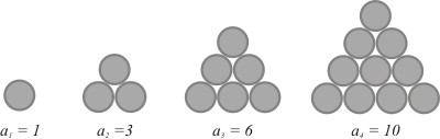
Ensimmäisen kolikon alle lisätään kaksi kolikkoa, jolloin toisessa vaiheessa saadaan \(a_2=3\) kolikkoa. Seuraavaksi tämän kolmion alle lisätään kolme uutta kolikkoa, joita on nyt yhteensä \(a_3=6\).
Etenemällä samaan tapaan huomataan, että esimerkiksi 10. kolmioluku saadaan laskemalla yhteen 10 ensimmäistä luonnollista lukua:
\[a_{10} = 1+2+3+\ldots+9+10.\] Yleinen kaava kolmiolukujonon termeille on \(a_{n} = 1+2+3+\ldots+(n-1)+n\). Kolmioluvuille käytetään yleensä merkintää \(T_n\) (T = 'Triangle').
Tämä motivoi seuraavaan määritelmään:
Määritelmä: Summajono
Olkoon \((a_n)_n, a_n: \mathbb{N}\to M\) jono joukossa \( M\), jossa on määritelty yhteenlasku. Merkitään \[a_1 + a_2 + a_3 + \ldots + a_{n-1} + a_n =: \sum_{k=1}^n a_k.\] Symboli \(\sum\) on kreikkalainen kirjain sigma. Summausindeksi \(k\) kasvaa alkuarvosta 1 loppuarvoon \(n\).
Summajono saadaan siis alkuperäisestä jonosta laskemalla alkupään termejä yhteen aina yksi termi eteenpäin. Varsinkin sarjojen kohdalla käytetään nimeä osasummajono.
Kolmiolukujen yleinen kaava voidaan siis kirjoittaa muodossa
\[T_n = \sum_{k=1}^n k\] ja kyseessä on luonnollisten lukujen jonon summajono.
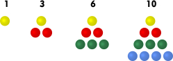
Esimerkki 3: Neliölukujen jono
Neliölukujen jono \((q_n)_n\) määritellään kaavalla \(q_n=n^2\). Tämän jonon termejä voidaan havainnollistaa asettelemalla kolikoita neliön muotoon.
Yksi mielenkiintoinen havainto on se, että kahden peräkkäisen kolmioluvun summa on aina neliöluku. Esimerkiksi \(3+1=4\) ja \(6+3=9\). Yleisesti määritelmiä käyttämällä
voidaan osoittaa, että
\[q_n=T_n + T_{n-1}.\]
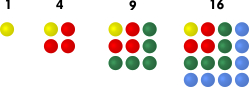
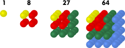
Esimerkki 4: Kuutiolukujen jono
Vastaavasti kuutiolukujen jono määritellään kaavalla \[a_n := n^3.\] Jonon ensimmäiset termit ovat silloin \((1,8,27,64,125,\ldots)\).
Esimerkki 5.
Olkoon \((q_n)_n\) with \(q_n := n^2\) neliölukujen jono \[\begin{aligned}(1,4,9,16,25,36,49,64,81,100 \ldots)\end{aligned}\] ja määritellään funktio \(\varphi(n) = 2n\). Jonosta \((q_{2n})_n\) saadaan \[\begin{aligned}(q_{2n})_n &= (q_2,q_4,q_6,q_8,q_{10},\ldots) \\ &= (4,16,36,64,100,\ldots).\end{aligned}\]
Määritelmä: Erotusjono (differenssijono)
Jonon \((a_{n})_{n}=a_{1},\, a_{2},\, a_{3},\ldots,\, a_{n},\ldots\) termeistä voidaan myös muodostaa peräkkäisten termien erotuksia: \[(a_{n+1}-a_{n})_{n}:=a_{2}-a_{1}, a_{3}-a_{2},\dots\] on nimeltään alkuperäisen jonon \((a_{n})_{n}\) ensimmäinen differenssijono.
Ensimmäisen differenssijonon ensimmäinen differenssijono on alkuperäisen jonon toinen differenssijono. sequence. Vastaavalla tavalla määritellään jonon \(n.\) differenssijono.
Esimerkki 6.
Tarkastellaan jonoa \((a_n)_n\), jossa \(a_n := \frac{n^2+n}{2}\), eli \[\begin{aligned}(a_n)_n &= (1,3,6,10,15,21,28,36,\ldots)\end{aligned}\] Olkoon \((b_n)_n\) sen 1. differenssijono. Silloin \[\begin{aligned}(b_n)_n &= (a_2-a_1, a_3-a_2, a_4-a_3,\ldots) \\ &= (2,3,4,5,6,7,8,9,\ldots)\end{aligned}\] Termin \((b_n)_n\) yleinen muoto on \[\begin{aligned}b_n &= a_{n+1}-a_{n} \\ &= \frac{(n+1)^2+(n+1)}{2} - \frac{n^2+n)}{2} \\ &= \frac{(n+1)^2+(n+1)-n^2 - n }{2} \\ &= \frac{(n^2+2n+1)+1-n^2}{2} \\ &= \frac{2n+2}{2} \\ &= n + 1.\end{aligned}\]
Eräitä tärkeitä jonoja
Eräät jonot ovat keskeisiä monille matemaattisille malleille ja niiden käytännön sovelluksille muilla aloilla kuten luonnontieteissä ja taloustieteissä.) Seuraavassa tarkastellaan kolme tällaista jonoa: aritmeettinen jono, geometrinen jono ja Fibonaccin lukujono.
Aritmeettinen jono
Aritmeettinen jono voidaan määritellä monella eri tavalla:Määritelmä A: Aritmeettinen jono
Jono \((a_{n})_{n}\) on aritmeettinen, jos sen peräkkäisten termien erotus \(d \in \mathbb{R}\) on vakio, t.s. \[a_{n+1}-a_{n}=d \text{ ja } d=vakio.\]
Huomautus: Aritmeettisen jonon eksplisiittinen kaava seuraa suoraan määritelmästä A: \[a_{n}=a_{1}+(n-1)\cdot d.\] Aritmeettisen jonon \(n.\) termi voidaan laskea myös palautuskaavan (eli rekursiokaavan) avulla: \[a_{n+1}=a_n + d.\]
Määritelmä B: Aritmeettinen jono
Jono \((a_{n})_{n}\) on aritmeettinen jono, jos sen ensimmäinen differenssijono on vakiojono.
Tämä määritelmä selventää myös aritmeettisen jonon nimen: Kolmen peräkkäisen termin keskimmäinen luku on kahden muun termin aritmeettinen keskiarvo; esimerkiksi
\[a_2 = \frac{a_1+a_3}{2}.\]
Esimerkki 1.
Luonnollisten lukujen jono \[(a_n)_n = (1,2,3,4,5,6,7,8,9,\ldots)\] on aritmeettinen, koska peräkkäisten termien erotus on \(d=1\).
Geometrinen jono
Myös geometrisella jonolla on useita erilaisia määritelmiä:
Määritelmä: Geometrinen jono
Jono \((a_{n})_{n}\) on geometrinen, jos kahden präkkäisen termin suhde on aina vakio \(q\in\mathbb{R}\), t.s. \[\frac{a_{n+1}}{a_{n}}=q \text{ kaikille } n\in\mathbb{N}.\]
Huomautus. Palautuskaava \(a_{n+1} = q\cdot a_n \) geometrisen jonon termeille ja myös eksplisiittinen lauseke \[a_n=a_1\cdot q^{n-1}\] seuraavat suoraan määritelmästä.
Myös tässä jonon nimityksellä on looginen tausta: Kolmen peräkkäisen termin keskimmäinen luku on aina kahden muun termin geometrinen keskiarvo; esimerkiksi \[a_2 = \sqrt{a_1\cdot a_3}.\]
Esimerkki 2.
Olkoon \(a\in\mathbf{R}\) ja \(q\neq 0\). Jono \((a_n)_n\), jolle \(a_n := aq^{n-1}\), eli \[\left( a_1, a_2, a_3, a_4,\ldots \right) = \left( a, aq, aq^2, aq^3,\ldots \right),\] on geometrinen jono. Jos \(a> 0\) ja \(q\geq1\), niin jono on aidosti kasvava. Jos \(a>0\) ja \(q<1\), niin se on aidosti vähenevä. Jonon alkioiden muodostama joukko \({a,aq,aq^2, aq^3}\) on äärellinen, jos \(q=1\) (jolloin sen ainoa alkio on \(a\)), muuten tämä joukko on ääretön.
Fibonaccin jono
Fibonaccin lukujono on kuuluisa sen biologisten sovellusten vuoksi. Se esiintyy mm.eliöiden populaation kasvun yhteydessä ja kasvien rakenteessa. Palautuskaavaan perustuva määritelmä on seuraava:
Määritelmä: Fibonaccin jono
Olkoon \(a_0 = a_1 = 1\) ja \[a_n := a_{n-2}+a_{n-1},\] kun \(n\geq2\). Jono \((a_n)_n\) on Fibonaccin lukujono. Jonon termit ovat Fibonaccin lukuja.
Jonon nimen takana on italialainen Leonardo Pisano (1200-luvulla), latinalaiselta nimeltään Filius Bonacci. Hän tutki kaniparien lisääntymistä idealisoidussa tilanteessa, jossa kanit eivät kuole ja kaikki vanhat sekä uudet parit lisääntyvät säännöllisin väliajoin. Näin hän päätyi jonoon \[(1,1,2,3,5,8,13,21,34,55,\ldots).\]
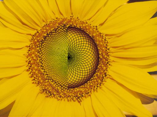
Esimerkki 3.
Auringonkukan kukat muodostuvat kahdesta spiraalista, jotka aukeavat keskeltä vastakkaisiin suuntiin: 55 spiraalia myötäpäivään ja 34 vastapäivään.
Myös ananashedelmän pinta käyttäytyy samalla tavalla. Siinä on 21 spiraalia yhteen suuntaan ja 34 vastakkaiseen. Myös joissakin kaktuksissa ja havupuiden kävyissä on samanlaisia rakenteita.
Suppeneminen, hajaantuminen ja raja-arvo
Tässä luvussa käsitellään jonon suppenemista. Aloitamme nollajonon käsitteestä ja siirrymme sen avulla yleiseen suppenemisen käsitteeseen.
Huomautus: Itseisarvo joukossa \(\mathbb{R}\)
Itseisarvofunktio \(x \mapsto |x|\) on keskeisessä asemassa jonojen suppenemisen tutkimisessa. Seuraavassa käydään läpi sen tärkeimmät ominaisuudet:
Määritelmä: Itseisarvo
Reaaliluvun \(x\in\mathbb{R}\) itseisarvo \(|x|\) on \[\begin{aligned}|x|:=\begin{cases}x, & \text{jos }x\geq0,\\ -x, & \text{jos }x<0.\end{cases}\end{aligned}\]
Itseisarvofunktion kuvaaja
Lause: Itseisarvon laskusääntöjä
Kaikille reaaliluvuille \(x,y\in\mathbb{R}\) pätee:
-
\(|x|\geq0,\)
-
\(|x|=0\) täsmälleen silloin, kun \(x=0.\)
-
\(|x\cdot y|=|x|\cdot|y|\) (multiplikatiivisuus)
-
\(|x+y|\leq|x|+|y|\) (kolmioepäyhtälö)
Kohdat 1.-3. Results follow directly from the definition and by dividing it up into separate cases of the different signs of \(x\) and \(y\)
Kohta 4. Tämä kohta voidaan todistaa neliöön korottamalla tai tutkimalla kaikki eri vaihtoehdot kuten alla.
Tapaus 1.
Olkoot \(x,y \geq 0\). Silloin \[\begin{aligned}|x+y|=x+y=|x|+|y|\end{aligned}\] ja kaava pätee.
Tapaus 2.Olkoot seuraavaksi \(x,y < 0\). Silloin \[\begin{aligned}|x+y|=-(x+y)=(-x)+ (-y)=|x|+|y|.\end{aligned}\]
Tapaus 3.Tutkitaan lopuksi tapaus \(x\geq 0\) and \(y<0\), joka jakaantuu kahteen alakohtaan:
-
Jos \(x \geq -y\), niin \(x+y\geq 0\) ja siten \(|x+y|=x+y\) määritelmän perusteella. Koska \(y<0\), niin \(y<-y\) ja sen vuoksi \(x+y < x-y\). Siis \[\begin{aligned}|x+y| = x+y < x-y = |x|+|y|.\end{aligned}\]
-
Jos \(x < -y\), niin \(x+y<0\), ja tällöin \(|x+y|=-(x+y)=-x-y\). Koska \(x\geq0\), niin \(-x < x\) ja siten \(-x-y\leq x-y\). Siispä \[\begin{aligned}|x+y| = -x-y \leq x-y = |x|+|y|.\end{aligned}\]
Jos \(x<0\) ja \(y\geq0\), niin väite seuraa samalla periaatteella kuin tapauksessa 3, kun vaihdetaan keskenään \(x\) ja \(y\).
\(\square\)
Nollajono
Määritelmä: Nollajono
Jono \((a_{n})_{n}\) on nollajono, jos jokaista \(\varepsilon>0,\) vastaa sellainen indeksi \(n_{0}\in\mathbb{N}\), että \[|a_{n}| < \varepsilon\] kaikille \(n\geq n_{0},\, n\in\mathbb{N}\). Tällöin sanotaan, että jono suppenee kohti nollaa.
Intuitiivisesti: Nollajonon termit menevät mielivaltaisen lähelle nollaa, kun jonossa mennään riittävän pitkälle.
Esimerkki 1.
Jono \((a_n)_n\), joka on määritelty kaavalla \(a_{n}:=\frac{1}{n}\), eli \[\left(a_{1},a_{2},a_{3},a_{4},\ldots\right):=\left(\frac{1}{1},\frac{1}{2},\frac{1}{3},\frac{1}{4},\ldots\right)\] on nimeltään harmoninen jono. Jonon termit ovat positiivisia kaikilla \(n\in\mathbb{N}\), mutta indeksin \(n\) kasvaessa jonon termit pienenevät yhä lähemmäksi
nollaa.
Jos esimerkiksi \(\varepsilon := \frac{1}{5000}\), niin valinnalla \(n_0 = 5001\) pätee \(a_n<\frac{1}{5000}=\varepsilon\) aina, kun \(n\geq n_0\).
Harmoninen jono suppenee kohti nollaa
Esimerkki 2.
Tarkastellaan jonoa \[(a_n)_n \text{ jossa } a_n:=\frac{1}{\sqrt{n}}.\] Olkoon \(\varepsilon := \frac{1}{1000}\). Tällöin valinnalla \(n_0=1000001\) kaikille termeille \(a_n\), joissa \(n\geq n_0\), pätee \(a_n < \frac{1}{1000}=\varepsilon\).
Note. Tutkittaessa nollajono-ominaisuutta täytyy tutkia mielivaltaista lukua \(\varepsilon \in \mathbb{R}\), jolle \(\varepsilon > 0\). Sen jälkeen yritetään valita sellainen indeksi \(n_0\), josta alkaen jokainen \(|a_n|\) on pienempi kuin \(\varepsilon\).
Esimerkki 3.
Tarkastellaan jonoa \((a_n)_n\), jossa \[a_n := \left( -1 \right)^n \cdot \frac{1}{n^2}.\]
Kerrointen \((-1)^n\) vuoksi jonon kaksi peräkkäistä termiä ovat aina erimerkkisiä; tällaista jonoa kutsutaan yleisemmin vuorottelevaksi jonoksi.
Osoitetaan, että kyseessä on nollajono. Määritelmän mukaan jokaista \(\varepsilon > 0\) täytyy vastata sellainen \(n_0 \in \mathbb{N}\), että epäyhtälö \[|a_n|< \varepsilon\] pätee kaikille niille termeille \(a_n\), joissa \(n\geq n_0\).
Olkoon siis \(\varepsilon > 0\) mielivaltainen. Koska epäyhtälön \( |a_n|< \varepsilon\) täytyy olla voimassa kaikille \(\varepsilon>0\), indeksin \(n_0\) täytyy riippua luvusta \(\varepsilon\). Tarkemmin: Epäyhtälön \[|a_{n_0}|=\left| \frac{1}{{n_0}^2} \right|= \frac{1}{{n_0}^2}<\varepsilon\] täytyy toteutua indeksillä \(n_0\). Ratkaistaan \(n_0\):
\[n_0 > \frac{1}{\sqrt{\varepsilon}}.\]. Mikä tahansa tämän ehdon toteuttava indeksi \(n_0\) kelpaa valinnaksi, kun \(\varepsilon > 0\) on alussa kiinnitetty.
Hajaantuvia esimerkkejä
Seuraavat kaavat eivät johda nollajonoon:
-
\(a_n = (-1)^n\)
-
\(a_n = (-1)^n \cdot n\)
Lause: Nollajonojen ominaisuuksia
Olkoot \((a_n)_n\) ja \((b_n)_n\) jonoja. Silloin pätee:
-
Jos \((a_n)_n\) on nollajono ja joko \(b_n = a_n\) tai \(b_n = -a_n\) kaikilla \(n\in\mathbb{N}\), niin \((b_n)_n\) on myös nollajono.
-
Jos \((a_n)_n\) on nollajono ja \(-a_n\leq b_n \leq a_n\) kaikilla \(n\in\mathbb{N}\), niin \((b_n)_n\) on myös nollajono.
-
Jos \((a_n)_n\) on nollajono, niin \((c\cdot a_n)_n\), \(c \in \mathbb{R}\), on myös nollajono.
-
Jos \((a_n)_n\) ja \((b_n)_n\) ovat nollajonoja, niin \((a_n + b_n)_n\) on myös nollajono.
Parts 1 and 2. If \((a_n)_n\) is a zero sequence, then according to the definition there is an index \(n_0 \in \mathbb{N}\), such that \(|a_n|<\varepsilon\) for every \(n\geq n_0\) and an arbitrary \(\varepsilon\in\mathbb{R}\). But then we have \(|b_n|\leq|a_n|<\varepsilon\); this proves parts 1 and 2 are correct.
Part 3. If \(c=0\), then the result is trivial. Let \(c\neq0\) and choose \(\varepsilon > 0\) such that \[\begin{aligned}|a_n|<\frac{\varepsilon}{|c|}\end{aligned}\] for all \(n\geq n_0\). Rearranging we get: \[\begin{aligned} |c|\cdot|a_n|=|c\cdot a_n|<\varepsilon\end{aligned}\]
Part 4.
Because \((a_n)_n\) is a zero sequence, by the definition we have \(|a_n|<\frac{\varepsilon}{2}\) for all \(n\geq n_0\). Analogously, for the zero sequence \((b_n)_n\) there is a \(m_0 \in \mathbb{N}\) with \(|b_n|<\frac{\varepsilon}{2}\) for all \(n\geq m_0\).
Then for all \(n > \max(n_0,m_0)\) it follows (using the triangle inequality) that: \[\begin{aligned}|a_n + b_n|\leq|a_n|+|b_n|<\frac{\varepsilon}{2}+\frac{\varepsilon}{2} = \varepsilon\end{aligned}\]
\(\square\)
Suppeneminen ja hajaantuminen
Nollajonoja voidaan käyttää tutkimaan jonojen suppenemista yleisemmin:
Määritelmä: Suppeneminen ja hajaantuminen
Jono \((a_{n})_{n}\) suppenee kohti raja-arvoa \(a\in\mathbb{R}\), jos jokaista \(\varepsilon>0\) vastaa sellainen \(n_{0}\), että \[|a_{n}-a| \lt \varepsilon \text{ kaikille niille }n\in\mathbb{N}_{0},\text{ joille }n\geq n_{0}.\]
Tämän kanssa on yhtäpitävää:
Jono \((a_{n})_{n}\) suppenee kohti raja-arvoa \(a\in\mathbb{R}\), jos \((a_{n}-a)_{n}\) on nollajono.
Esimerkki 4.
Tarkastellaan jonoa \((a_n)_n\), jossa \[a_n=\frac{2n^2+1}{n^2+1}.\] Laskemalla jonon termejä suurilla \(n\), huomataan, että ilmeisesti \( a_n\to 2\), kun \(n \to \infty\), joten jonon raja-arvo voisi olla \(a=2\).
For a vigorous proof, we show that for every \(\varepsilon > 0\) there exists an index \(n_0\in\mathbb{N}\), such that for every term \(a_n\) with \(n>n_0\) the following relationship holds: \[\left| \frac{2n^2+1}{n^2+1} - 2\right| < \varepsilon.\]
Firstly we estimate the inequality: \[\begin{aligned}\left|\frac{2n^2+1}{n^2+1}-2\right| =&\left|\frac{2n^2+1-2\cdot\left(n^2+1\right)}{n^2+1}\right| \\ =&\left|\frac{2n^2+1-2n^2-2}{n^2+1}\right| \\ =&\left|-\frac{1}{n^2+1}\right| \\ =&\left|\frac{1}{n^2+1}\right| \\ <&\frac{1}{n}.\end{aligned}\]
Now, let \(\varepsilon > 0\) be an arbitrary constant. We then choose the index \(n_0\in\mathbb{N}\), such that \[n_0 > \frac{1}{\varepsilon} \text{, or equivalently, } \frac{1}{n_0} < \varepsilon.\] Finally from the above inequality we have: \[\left|\frac{2n^2+1}{n^2+1}-2\right| < \frac{1}{n} < \frac{1}{n_0} < \varepsilon,\] Thus we have proven the claim and so by definition \(a=2\) is the limit of the sequence.
\(\square\)
Jos jono suppenee, niin sillä voi olla vain yksi raja-arvo.
Lause: Raja-arvon yksikäsitteisyys
Oletetaan, että jono \((a_{n})_{n}\) suppenee kohti raja-arvoa \(a\in\mathbb{R}\) ja kohti raja-arvoa \(b\in\mathbb{R}\).
Silloin \(a=b\).
Assume \(a\ne b\); choose \(\varepsilon\in\mathbb{R}\) with \(\varepsilon:=\frac{1}{3}|a-b|.\) Then in particular \([a-\varepsilon,a+\varepsilon]\cap[b-\varepsilon,b+\varepsilon]=\emptyset.\)
Because \((a_{n})_{n}\) converges to \(a\), there is, according to the definition of convergence, a index \(n_{0}\in\mathbb{N}\) with \(|a_{n}-a|< \varepsilon\) for \(n\geq n_{0}.\) Furthermore, because \((a_{n})_{n}\) converges to \(b\) there is also a \(\widetilde{n_{0}}\in\mathbb{N}\) with \(|a_{n}-b|< \varepsilon\) for \(n\geq\widetilde{n_{0}}.\) For
\(n\geq\max\{n_{0},\widetilde{n_{0}}\}\) we have:
\[\begin{aligned}\varepsilon\ = &\ \frac{1}{3}|a-b| \Rightarrow\\
3\varepsilon\ = &\ |a-b|\\
= &\ |(a-a_{n})+(a_{n}-b)|\\
\leq &\ |a_{n}-a|+|a_{b}-b|\\
< &\ \varepsilon+\varepsilon=2\varepsilon,\end{aligned}\] Consequently we have obtained \(3\varepsilon\leq2\varepsilon\), which is a contradiction as \(\varepsilon>0\).
Therefore the assumption must be wrong, so \(a=b\).
\(\square\)
Määritelmä: Raja-arvo
Suppenevan jonon raja-arvolle käytetään merkintöjä\[a_{n}\rightarrow a,\text{ tai }\lim_{n\rightarrow\infty}a_{n}=a.\] Määritelmä on yksikäsitteinen yllä
olevan lauseen perusteella. Jos jonolla ei ole raja-arvoa, niin se hajaantuu.
Lause: Rajoitettu jono
Suppeneva jono \((a_n)_n\) on rajoitettu, t.s. on olemassa sellainen vakio \(C\in\mathbb{R}\) että
\[|a_n| \lt C\] kaikilla
\(n\in\mathbb{N}\).
We assume that the sequence \((a_n)_n\) has the limit \(a\). By the definition of convergence, we have that \(|a_n - a|<\varepsilon\) for all \(\varepsilon \in \mathbb{R}\) and \(n\geq n_0\). Choosing \(\varepsilon = 1\) gives:
\[\begin{aligned}|a_n|-|a|&\ \leq |a_n -a| \\
&\ < 1,\end{aligned}\] And therefore also \(|a_n|\leq |a|+1\).
Thus for all \(n\in \mathbb{N}\): \[|a_n|\leq \max \left\{ |a_1|,|a_2|,\ldots,|a_{n_0}|,|a|+1 \right\}=:r\]
\(\square\)
Suppenevien jonojen ominaisuuksia
Lause: Osajono
Olkoon \((a_{n})_{n}\) suppeneva jono, jolle \(a_{n}\rightarrow a\) ja olkoon \((a_{\varphi(n)})_{n}\) jonon \((a_{n})_{n}\) osajono. Silloin \((a_{\varphi(n)})_{n}\rightarrow a\).
Sanallisesti: Suppenevan jonon kaikki osajonot suppenevat kohti alkuperäisen jonon raja-arvoa.
By the definition of a subsequence \(\varphi(n)\geq n\). Because \(a_{n}\rightarrow a\) it is implicated that \(|a_{n}-a|<\varepsilon\) for \(n\geq n_{0}\), therefore \(|a_{\varphi(n)}-a|<\varepsilon\) for these indices \(n\).
\(\square\)
Lause: Laskusääntöjä
Olkoot \((a_{n})_{n}\) ja \((b_{n})_{n}\) suppenevia jonoja, joille \(a_{n}\rightarrow a\) ja \(b_{n}\rightarrow b\). Silloin kaikille \(\lambda, \mu \in \mathbb{R}\) pätee:
-
\(\lambda \cdot (a_n)+\mu \cdot (b_n) \to \lambda \cdot a + \mu \cdot b\)
-
\((a_n)\cdot (b_n) \to a\cdot b\)
Sanallisesti: Suppenevien jonojen summat ja tulot ovat suppenevia jonoja.
Part 1. Let \(\varepsilon > 0\). We must show, that for all \(n \geq n_0\) it follows that: \[|\lambda \cdot a_n + \mu \cdot b_n - \lambda \cdot a - \mu \cdot b| < \varepsilon.\] The left hand side we estimate using: \[|\lambda (a_n-a)+\mu (b_n - b)| \leq |\lambda|\cdot|a_n-a|+|\mu|\cdot|b_n-b|.\]
Because \((a_n)_n\) and \((b_n)_n\) converge, for each given \(\varepsilon > 0\) it holds true that: \[\begin{aligned}|a_n - a| <\ \varepsilon_1 := &\ \textstyle \frac{\varepsilon}{2|\lambda|} \text{ for all }n\geq n_0\\ |b_n - b| <\ \varepsilon_2 := &\ \textstyle \frac{\varepsilon}{2|\mu|} \text{ for all }n\geq n_1\end{aligned}\]
Therefore \[\begin{aligned}|\lambda|\cdot|a_n-a|+|\mu|\cdot|b_n-b| < &\ |\lambda|\varepsilon_1 + |\mu|\varepsilon_2 \\ = &\ \textstyle{ \frac{\varepsilon}{2} + \frac{\varepsilon}{2} } = \varepsilon\end{aligned}\] for all numbers \(n \geq \max \{n_0,n_1\}\). Therefore the sequence \[\left( \lambda \left( a_n - a \right) + \mu \left( b_n - b \right) \right)_n\] is a zero sequence and the desired inequality is shown.
Part 2. Let \(\varepsilon > 0\). We have to show, that for all \(n > n_0\) \[|a_n b_n - a b| < \varepsilon.\] Furthermore an estimation of the left hand side follows: \[\begin{aligned} |a_n b_n - a b| =&\ |a_n b_n - a b_n + a b_n - ab| \\ \leq &\ |b_n|\cdot|a_n-a| + |a|\cdot|b_n - b|.\end{aligned}\] We choose a number \(B\), such that \(|b_n| \lt b\) for all \(n\) and \(|a| \lt b\). Such a value of \(B\) exists by the Theorem of convergent sequences being bounded. We can then use the estimation: \[\begin{aligned}|b_n|\cdot|a_n-a| + |a|\cdot|b_n - b| <&\ B \cdot \left(|a_n - a| + |b_n - b| \right).\end{aligned}\] For all \(n>n_0\) we have \(|a_n - a|<\frac{\varepsilon}{2\cdot B}\) and \(|b_n - b|<\frac{\varepsilon}{2\cdot B}\), and - putting everything together - the desired inequality it shown.
\(\square\)
2. Sarjat
Suppeneminen
Suppeneminen
Jonosta \((a_k)\) voidaan muodostaa sen osasummia asettamalla \[s_n =a_1+a_2+\dots+a_n.\]
Jos osasumminen jonolla \((s_n)\) on raja-arvo \(s\in \mathbb{R}\), niin luvuista \((a_k)\) muodostettu sarja suppenee ja sen summa on \(s\). Tällöin merkitään \[ a_1+a_2+\dots =\sum_{k=1}^{\infty} a_k = \lim_{n\to\infty}\underbrace{\sum_{k=1}^{n} a_k}_{=s_{n}} = s. \]
Indeksöinti
Osasummat kannattaa indeksöidä samalla tavalla kuin alkuperäinen jono \((a_k)\); esimerkiksi jonon \((a_k)_{k=0}^{\infty}\) osasummat ovat \(s_0= a_0, s_1=a_0+a_1\) jne.
Sarjaan voidaan tehdä indeksinsiirtoja ilman että varsinainen sarja muuttuu: \[\sum_{k=1}^{\infty} a_k =\sum_{k=0}^{\infty} a_{k+1} = \sum_{k=2}^{\infty} a_{k-1}.\]
Konkreettinen esimerkki: \[\sum_{k=1}^{\infty} \frac{1}{k^2}=1+\frac{1}{4}+\frac{1}{9}+\dots= \sum_{k=0}^{\infty} \frac{1}{(k+1)^2}\]
Kokeile!
Laske sarjan \(\displaystyle\sum_{k=0}^{\infty}a_{k}\) osasummia:
sarjan \(k.\) termi: , aloita summaus kohdasta
Sarjan hajaantuminen
Sarja, joka ei suppene, on hajaantuva. Tämä voi tapahtua kolmella eri tavalla:
- sarjan osasummat kasvavat rajatta kohti ääretöntä
- sarjan osasummat pienenevät rajatta kohti miinus ääretöntä
- osasummien jono heilahtelee niin, ettei sillä ole raja-arvoa.
Hajaantuvan sarjan kohdalla merkintä \(\displaystyle\sum_{k=1}^{\infty} a_k\) ei oikeastaan tarkoita mitään (se ei ole reaaliluku). Tällöin voidaan tulkita, että merkintä tarkoittaa osasummien jonoa, joka on aina hyvin määritelty.
Perustuloksia
Geometrinen sarja
Geometrinen sarja \[\sum_{k=0}^{\infty} aq^k\] suppenee, jos \(|q|<1\) (tai \(a=0\)), jolloin sen summa on \(\frac{a}{1-q}\). Jos \(|q|\ge 1\), niin sarja hajaantuu.
Todistus. Osasummille on voimassa
\[\sum_{k=0}^{n} aq^k =\frac{a(1-q^{n+1})}{1-q},\] josta väite seuraa.
\(\square\)
Yleisemmin \[\sum_{k=i}^{\infty} aq^k = \frac{aq^i}{1-q} = \frac{\text{sarjan 1. termi}}{1-q},\text{ jos } |q|<1.\]
Esimerkki 1.
Määritä sarjan \[\sum_{k=1}^{\infty}\frac{3}{4^{k+1}}\] summa.
Ratkaisu. Koska \[\frac{3}{4^{k+1}} = \frac{3}{4}\cdot \left( \frac{1}{4}\right)^k,\] niin kyseessä on geometrinen sarja. Sen summa on \[\frac{3}{4}\cdot \frac{1/4}{1-1/4} = \frac{1}{4}.\]
Laskusääntöjä
Suppenevien sarjojen ominaisuuksia:
- \(\displaystyle{\sum_{k=1}^{\infty} (a_k+b_k) = \sum_{k=1}^{\infty} a_k + \sum_{k=1}^{\infty} b_k}\)
- \(\displaystyle{\sum_{k=1}^{\infty} (c\, a_k) = c\sum_{k=1}^{\infty} a_k}\), kun \(c\in \mathbb{R}\) on vakio
Todistus. Nämä seuraavat vastaavista tuloksista jonojen raja-arvolle.
\(\square\)
Huomautus: Sarjoilla ei ole jonojen kaltaista tulosääntöä, koska jo kahden termin summille \[(a_1+a_2)(b_1+b_2) \neq a_1b_1 +a_2b_2.\] Tulosäännön oikea muoto on sarjojen Cauchy-tulo, jossa myös ristitermit otetaan huomioon.
Katso esimerkiksi https://en.wikipedia.org/wiki/Cauchy_product
Lause 1.
Jos sarja \(\displaystyle{\sum_{k=1}^{\infty} a_k}\) suppenee, niin \[\displaystyle{\lim_{k\to \infty} a_k =0}.\]
Kääntäen: Jos \[\displaystyle{\lim_{k\to \infty} a_k \neq 0},\] niin sarja \(\displaystyle{\sum_{k=1}^{\infty} a_k}\) hajaantuu.
Todistus.
Jos sarjan summa on \(s\), niin \(a_k=s_k-s_{k-1}\to s-s=0\).
\(\square\)
Huomautus: Ominaisuutta \(\lim_{k\to \infty} a_k = 0\) ei voi käyttää sarjan suppenemisen osoittamiseen; vrt. seuraavat esimerkit. Tämä on eräs yleisimmistä päättelyvirheistä sarjojen kohdalla!
Esimerkki
Tutki sarjan \[\sum_{k=1}^{\infty} \frac{k}{k+1} = \frac{1}{2}+\frac{2}{3}+\frac{3}{4}+\dots\] suppenemista.
Ratkaisu. Sarjan yleisen termin raja-arvo on \[\lim_{k\to\infty}\frac{k}{k+1} = 1.\] Koska raja-arvo ei ole nolla, niin sarja hajaantuu.
Harmoninen sarja
Harmoninen sarja \[\sum_{k=1}^{\infty} \frac{1}{k} = 1+\frac{1}{2}+\frac{1}{3}+\dots\] hajaantuu, vaikka yleisen termin \(a_k=1/k\) raja-arvo on nolla.
Tämän klassisen tuloksen todisti ensimmäisenä 14. vuosisadalla Nicole Oresme, jonka jälkeen monia muitakin perusteluja on keksitty. Tässä esimerkkinä kaksi erilaista päättelyä.
i) Alkeellinen todistus. Oletetaan, että sarja suppenee ja yritetään johtaa tästä ristiriita. Olkoon siis \(s\in\mathbb{R}\) harmonisen sarjan summa: \(s = \sum_{k=1}^{\infty}1/k\). Tällöin
\[
s = \left(\color{#4334eb}{1} + \color{#eb7134}{\frac{1}{2}}\right) + \left(\color{#4334eb}{\frac{1}{3}} +
\color{#eb7134}{\frac{1}{4}}\right) + \left(\color{#4334eb}{\frac{1}{5}} + \color{#eb7134}{\frac{1}{6}}\right) + \dots
= \sum_{k=1}^{\infty}\left(\color{#4334eb}{\frac{1}{2k-1}} + \color{#eb7134}{\frac{1}{2k}}\right).
\] Selvästi
\[
\color{#4334eb}{\frac{1}{2k-1}} > \color{#eb7134}{\frac{1}{2k}} > 0 \text{ kaikille }k\ge 1~\Rightarrow~\sum_{k=1}^{\infty}\color{#4334eb}{\frac{1}{2k-1}} > \sum_{k=1}^{\infty}\color{#eb7134}{\frac{1}{2k}} = \frac{s}{2},
\] joten \[
s = \sum_{k=1}^{\infty}\color{#4334eb}{\frac{1}{2k-1}} + \sum_{k=1}^{\infty}\color{#eb7134}{\frac{1}{2k}} = \sum_{k=1}^{\infty}\color{#4334eb}{\frac{1}{2k-1}} + \frac{1}{2}\underbrace{\sum_{k=1}^{\infty}\frac{1}{k}}_{=s}.
\]
\[
= \sum_{k=1}^{\infty}\color{#4334eb}{\frac{1}{2k-1}} + \frac{s}{2} > \sum_{k=1}^{\infty}\color{#eb7134}{\frac{1}{2k}} + \frac{s}{2} = \frac{s}{2} + \frac{s}{2} = s.
\] Päädyimme siis epäyhtälöön \(s>s\), joka on ristiriita. Alkuperäinen oletus suppenemisesta on siis väärä, joten sarja hajaantuu.
\(\square\)
ii) Todistus integraalin avulla: Pylvään korkeuksia \(1/k\) vastaavan histogrammin alapuolelle jää funktion \(f(x)=1/(x+1)\) kuvaaja, joten pinta-aloja vertaamalla saadaan
\[\sum_{k=1}^{n} \frac{1}{k} \ge \int_0^n\frac{dx}{x+1} =\ln(n+1)\to\infty, \] kun \(n\to\infty\).
\(\square\)
Positiiviset sarjat
Sarjan summan laskeminen on usein vaikeata ja monesti jopa mahdotonta, jos vaatimuksena on summan eksplisiittinen lauseke. Moniin sovelluksiin riittää myös summan likiarvo, mutta sitä ennen olisi syytä selvittää, onko sarja suppeneva vai hajaantuva.
Sarja \(\displaystyle{\sum_{k=1}^{\infty} p_k}\) on positiivinen (tai positiiviterminen), jos \(p_k > 0\) kaikilla \(k\).
Positiivisten sarjojen suppeneminen on hyvin selväpiirteistä:
Lause 2.
Positiivinen sarja suppenee täsmälleen silloin, kun sen osasummien jono on ylhäältä rajoitettu.
Syy: Osasummien jono on nouseva.
Esimerkki
Osoita, että superharmonisen sarjan \[\sum_{k=1}^{\infty}\frac{1}{k^2}\] osasummille pätee \(s_n<2\) kaikilla \(n\), joten sarja suppenee.
Ratkaisu. Ratkaisu perustuu epäyhtälöön \[\frac{1}{k^2} < \frac{1}{k(k-1)} = \frac{1}{k-1}-\frac{1}{k},\] kun \(k\ge 2\), koska sen mukaan \[\sum_{k=1}^n\frac{1}{k^2} < 1+ \sum_{k=2}^n\frac{1}{k(k-1)} =2-\frac{1}{n}< 2\] kaikilla \(n\ge 2\).
Tämän päättelyn voi tehdä myös integraalin avulla.
Leonhard Euler selvitti vuonna 1735, että sarjan summa on \(\pi^2/6\). Perusteluna hän käytti sinifunktion sarja- ja tulokehitelmien vertailua.
Itseinen suppeneminen
Määritelmä
Sarja \(\displaystyle{\sum_{k=1}^{\infty} a_k}\) suppenee itseisesti, jos positiivinen sarja \(\sum_{k=1}^{\infty} |a_k|\) suppenee.
Lause 3.
Itseisesti suppeneva sarja suppenee (tavallisessa mielessä) ja \[\left| \sum_{k=1}^{\infty} a_k \right| \le \sum_{k=1}^{\infty} |a_k|.\]
Tämä on erikoistapaus majoranttiperiaatteesta, josta lisää myöhemmin.
Todistus.
Oletetaan, että \(\sum_k |a_k|\) suppenee. Tarkastellaan erikseen sarjan \(\sum_k a_k\) positiivista ja negatiivista osaa: Olkoon \[b_k=\max (a_k,0)\ge 0 \text{ ja } c_k=-\min (a_k,0)\ge 0.\] Koska \(b_k,c_k\le |a_k|\), niin positiiviset sarjat \(\sum b_k\) ja \(\sum c_k\) suppenevat lauseen 2 perusteella. Lisäksi \(a_k=b_k-c_k\), joten \(\sum a_k\) suppenee kahden suppenevan sarjan erotuksena.
\(\square\)
Esimerkki
Tutki vuorottelevan (= etumerkit vaihtelevat vuorotellen + ja -) sarjan \[\sum_{k=1}^{\infty}\frac{(-1)^{k+1}}{k^2}=1-\frac{1}{4}+\frac{1}{9}-\dots\] suppenemista.
Ratkaisu. Koska \[\displaystyle{\left| \frac{(-1)^{k+1}}{k^2}\right| =\frac{1}{k^2}}\] ja superharmoninen sarja \[\sum_{k=1}^{\infty}\frac{1}{k^2}\] suppenee, niin tutkittava sarja suppenee itseisesti, ja sen vuoksi myös tavallisessa mielessä.
Vuorotteleva harmoninen sarja
Itseinen suppeneminen ei kuitenkaan tarkoita samaa kuin tavallinen suppeneminen:
Esimerkki
Vuorotteleva harmoninen sarja \[\sum_{k=1}^{\infty}\frac{(-1)^{k+1}}{k} = 1-\frac{1}{2}+\frac{1}{3}-\frac{1}{4}+\dots\] suppenee, mutta ei itseisesti.
(Idea) Piirretään osasummajonon \((s_n)\) kuvaaja, josta huomataan, että parillisten ja parittomien indeksien osasummat \(s_{2n}\) ja \(s_{2n+1}\) ovat monotonisia ja suppenevat kohti samaa raja-arvoa.
Sarjan summa on \(\ln 2\), joka saadaan selville integroimalla geometrisen sarjan summakaavaa.
pisteet on yhdistetty janoilla havainnollisuuden vuoksi
Suppenemistestejä
Vertailutestit
Edelliset tarkastelut yleistyvät seuraavalla tavalla:
Lause 4.
(Majoranttiperiaate) Jos \(|a_k|\le p_k\) kaikilla \(k\) ja
\(\sum_{k=1}^{\infty} p_k\) suppenee, niin myös \(\sum_{k=1}^{\infty} a_k\) suppenee.
(Minoranttiperiaate) Jos \(0\le p_k \le a_k\) kaikilla \(k\) ja \(\sum p_k\) hajaantuu, niin myös \(\sum a_k\) hajaantuu.
Majorantin todistus. Koska \[a_k=|a_k|-(|a_k|-a_k)\] ja \[0\le |a_k|-a_k \le 2|a_k|,\] niin \(\sum a_k\) on suppeneva kahden suppenevan sarjan erotuksena. Tässä käytetään aikaisempaa lausetta 2 positiivisille sarjoille; kyseessä ei ole kehäpäättely!
Minorantin todistus. Oletuksista seuraa, että sarjan \(\sum a_k\) osasummat kasvavat rajatta, joten sarja hajaantuu.
\(\square\)
Esimerkki
Tutki sarjojen \[
\sum_{k=1}^{\infty} \frac{1}{1+k^3} \ \text{ ja }\
\sum_{k=1}^{\infty} \frac{1}{\sqrt{k}}
\] suppenemista.
Ratkaisu. Koska\[0<\frac{1}{1+k^3} < \frac{1}{k^3}\le \frac{1}{k^2}\] kaikilla \(k\in \mathbb{N}\), niin ensimmäinen sarja suppenee majoranttiperiaatteen nojalla.
Toisaalta \[\displaystyle{\frac{1}{\sqrt{k}}\ge \frac{1}{k}}\] kaikilla \(k\in\mathbb{N}\), joten toisella sarjalla on hajaantuva harmoninen minorantti, joten se hajaantuu.
Suhdetesti
Käytännössä eräs parhaista tavoista tutkia suppenemista on suhdetesti, jossa sarjan peräkkäisten termien käyttäytymistä verrataan sopivaan geometriseen sarjaan:
Lause 5a.
Oletetaan, että on olemassa sellainen vakio \(0< Q < 1\), että \[ \left| \frac{a_{k+1}}{a_k} \right| \le Q\] jostakin indeksistä \(k\ge k_0\) alkaen.
Tällöin sarja \(\sum a_k\) suppenee (ja sen "suppenemisnopeus"\ on samaa luokkaa kuin geometrisella sarjalla \(\sum Q^k\), tai jopa parempi).
Koska sarjan alkuosa ei vaikuta suppenemiseen (mutta se vaikuttaa toki summaan!), niin voidaan olettaa epäyhtälön pätevän kaikilla indekseillä \(k\).
Tästä seuraa, että \[|a_{k}|\le Q|a_{k-1}|\le Q^2|a_{k-2}|\le \dots\le Q^k|a_0|,\] joten sarjalla on geometrinen majorantti, ja se suppenee.
\(\square\)
Suhdetestin raja-arvomuoto
Lause 5b.
Oletetaan, että raja-arvo \[\lim_{k\to \infty} \left| \frac{a_{k+1}}{a_k} \right| = q\] on olemassa. Silloin sarja \(\sum a_k\) \[ \begin{cases}\text{suppenee,} & \text{ jos } 0\le q< 1,\\ \text{hajaantuu,} & \text{ jos } q > 1,\\ \text{voi olla suppeneva tai haantuva,} & \text{ jos } q=1. \end{cases} \]
(Idea) Geometriselle sarjalle kahden peräkkäisen termin suhde on täsmälleen \(q\). Suhdetestin mukaan muidenkin sarjojen suppenemista voidaan (usein) tutkia samalla periaatteella, kun suhdeluku \(q\) korvataan tällä raja-arvolla.
Valitaan raja-arvon määritelmässä \(\varepsilon =(1-q)/2>0\). Silloin jostakin indeksistä \(k\ge k_{\varepsilon}\) alkaen pätee \[ |a_{k+1}/a_k| < q + \varepsilon = (q+1)/2 = Q < 1, \] ja väite seuraa lauseesta 4.
Tapauksessa \(q>1\) sarjan yleinen termi ei lähesty nollaa, joten sarja hajaantuu.
Viimeinen tapaus \(q=1\) ei sisällä mitään informaatiota (eikä myöskään todistettavaa).
Tämä tapaus esiintyy sekä harmonisen (\(a_k=1/k\), hajaantuu!) että yliharmonisen (\(a_k=1/k^2\), suppenee!) sarjan kohdalla. Näissä tapauksissa suppenemista täytyy tutkia joillakin muilla menetelmillä, kuten aikaisemmin tehtiin.
\(\square\)
Esimerkki
Onko sarja \[\sum_{k=1}^{\infty}\frac{(-1)^{k+1}k}{2^k}= \frac{1}{2}-\frac{2}{4}+\frac{3}{8}-\dots\] suppeneva?
Ratkaisu. Tässä \(a_k=(-1)^{k+1}k/2^k\), joten \[ \left| \frac{a_{k+1}}{a_k}\right| = \left| \frac{(-1)^{k+2}(k+1)/2^{k+1}}{(-1)^{k+1}k/2^k}\right| =\frac{k+1}{2k} =\frac{1}{2}+\frac{1}{2k}\to \frac{1}{2} < 1, \] kun \(k\to\infty\). Suhdetestin perusteella sarja suppenee.
3. Continuity
Table of Content
In this section we define a limit of a function \(f\colon S\to \mathbb{R}\) at a point \(x_0\). It is assumed that the reader is already familiar with limit of a sequence, the real line and the general concept of a function of one real variable.
Limit of a function
For a subset of real numbers, denoted by \(S\), assume that \(x_0\) is such point that there is a sequence of points \((x_k)\in S\) such that \(x_k\to x_0\) as \(k\to \infty\). Here the set \(S\) is often the set of all real numbers, but sometimes an interval (open or closed).
Example 1.
Note that it is not necessary for \(x_0\) to be in \(S\). For example, the sequence \(x_k = 1/k\to 0\) as \(k\to \infty\) in \(S=]0,2[\), and \(x_k\in S\) for all \(k=1,2,\ldots\) but \(0\) is not in \(S\).
Limit of a function
We consider a function \(f\) defined in the set \(S\). Then we define the limit of the function \(f\colon S\to \mathbb{R}\) at \(x_0\) as follows.
Definition 1: Limit of a function
Suppose that \(S\subset \mathbb{R}\) and \(f\colon S\to \mathbb{R}\) is a function. Then we say that \(f\) has a limit \(y_{0}\) at \(x_{0}\), and write \[\lim_{x \to x_{0}}f(x)=y_{0},\] if, \(f(x_{k})\to y_{0}\) as \(k\to \infty\) for every sequence \((x_{k})\) in \(S\setminus\{x_0\}\), such that \(x_{k}\to x_{0}\) as \(k\to \infty\).
Example 2.
The function \(f\colon \mathbb{R} \to \mathbb{R}\) defined by \(f(x)=x^2\) has a limit \(0\) at the point \(x=0\).
Function \(y=x^2\).
Example 3.
The function \(g\colon\mathbb{R}\to \mathbb{R}\) defined by \[g(x)= \left\{\begin{array}{rl}0 & \text{ for }x<0, \\ 1 & \text{ for }x\ge 0.\end{array}\right.\] does not have a limit at the point \(x=0\). To formally prove this, take sequences \((x_k)\), \((y_k)\) defined by \(x_k=1/k\) and \(y_k=-1/k\) for \(k=1,2,\ldots\). Then the both sequences are in \(S=\mathbb{R}\), but \(f(x_k)=1\) and \(f(y_k)=0\) for any \(k\).
Function \[g(x)= \left\{\begin{array}{rl}0 & \text{ for }x<0, \\ 1 & \text{ for }x\ge 0.\end{array}\right.\]
Example 4.
The function \(f(x)=x \sin(1/x)\), \(x>0\) does have the limit \(0\) at \(0\).
Function \(y=x\sin(1/x)\) for \(x>0\).
Example 5.
The function \(g(x)= \sin(1/x)\), \(x>0\) does not have a limit at \(0\).
Function \(y=\sin(1/x)\) for \(x>0\).
One-sided limits
An important property of limits is that they are always unique. That is, if \(\lim_{x\to x_0} f(x)=a\) and \(\lim_{x\to x_0} f(x)=b\), then \(a=b\). Although a function may have only one limit at a given point, it is sometimes useful to study the behavior of the function when \(x_k\) approaches the point \(x_0\) from the left or the right side. These limits are called the left and the right limit of the function \(f\) at \(x_0\), respectively.
Definition 2: One-sided limits
Suppose \(S\) is a set in \(\mathbb{R}\) and \(f\) is a function defined on the set \(S\setminus\{x_0\}\). Then we say that \(f\) has a left limit \(y_{0}\) at \(x_{0}\), and write \[\lim_{x \to x_{0}-}f(x)=y_{0},\] if, \(f(x_{k})\to y_{0}\) as \(k\to \infty\) for every sequence \((x_{k})\) in the set \(S\cap ]-\infty,x_0[ =\{ x\in S : x < x_0 \}\), such that \(x_{k}\to x_{0}\) as \(k\to \infty\).
Similarly, we say that \(f\) has a right limit \(y_{0}\) at \(x_{0}\), and write \[\lim_{x \to x_{0}+}f(x)=y_{0},\] if, \(f(x_{k})\to y_{0}\) as \(k\to \infty\) for every sequence \((x_{k})\) in the set \(S\cap ]x_0,\infty[ =\{ x\in S : x_0 < x \}\), such that \(x_{k}\to x_{0}\) as \(k\to \infty\).
Theorem 1: Limit of a function
A function \(f\colon S\to \mathbb{R}\) has a limit \(y_0\) at the point \(x_0\) if and only if \[\lim_{x \to x_{0}-}f(x)= \lim_{x \to x_{0}+}f(x)=y_{0}.\]
Example 6.
The sign function \[\mathrm{sgn}(x)= \frac{x}{|x|}\] is defined on \(S= \mathbb{R}\setminus 0\). Its left and right limits at \(0\) are \[\lim_{x\to 0-} \mathrm{sgn}(x)= -1,\qquad \lim_{x\to 0+} \mathrm{sgn}(x)= 1.\] However, the function \(\mathrm{sgn}(x)\) does not have a limit at \(0\).
Function \(y = \frac{x}{|x|}\).
Example 7.
Function \(f: \mathbb{R}\setminus 0 \to \mathbb{R}\) \[f(x) = \frac{1}{x}\] does not have one-sided limits at 0.
Limit rules
The following limit rules are immediately obtained from the definition and basic algebra of real numbers.
Theorem 2: Limit rules
Let \(c\in \mathbb{R}, \lim_{x\to x_{0}} f(x)=a\) and \(\lim_{x\to x_{0}} g(x)=b.\) Then
- \(\lim_{x\to x_{0}} (cf)(x)=ca\),
- \(\lim_{x\to x_{0}} (f+g)(x)=a+b\),
- \(\lim_{x\to x_{0}} (fg)(x)=ab\),
- \(\lim_{x\to x_{0}} (f/g)(x)=a/b \ (\text{if} \ b \neq 0)\).
Example 8.
Finding limits by calculating \(f(x_0)\):
a) \[\lim_{x\to 2}(5x-3)=10-3=7.\]
b) \[\lim_{x\to -2}\frac{3x+2}{x+5} = \frac{-6+2}{-2+5}=-\frac{4}{3}.\]
c) \[\lim_{x\to 2} \frac{x^2-4}{x-2} = \lim_{x\to 2} \frac{(x+2)(x-2)}{x-2} = \lim_{x\to 2}(x+2) = 4.\]
Limits and continuity
In this section, we define continuity of the function. The intutive idea behind continuity is that the graph of a continuous function is a connected curve. However, this is not sufficient as a mathematical definition for several reasons. For example, by using this definition, one cannot easily decide if \(\tan(x)\) is a continuous function or not.
For continuity of a function \(f\) at a given point \(x_0\), it is required that:
\(f(x_0)\) is defined,
\(\lim_{x \to x_0} f(x)\) exists (and is finite),
\(\lim_{x \to x_0} f(x) = f(x_0)\).
In other words:
Definition 2: Continuity
A function \(f\colon S\to \mathbb{R}\) is continuous at a point \(x_{0}\in S\), if \[\lim_{x\to x_{0}}f(x)=f(x_{0}).\] A function \(f\colon S\to \mathbb{R}\) is continuous, if it is continuous at every point \(x_{0}\in S\).
Example 1.
Let \(c\in \mathbb{R}\). Functions \(f,g,h\) defined by \(f(x)=c\), \(g(x)=x\), \(h(x)=|x|\) are continuous at every point \(x\in \mathbb{R}\).
Why? If \(x_{k}\to x_{0}\), then \(f(x_{k})=c\) and \(\lim_{k\to \infty}f(x_k)= c=f(x_{0})\). For \(g\), we have \(g(x_{k})=x_{k}\) and hence, \(\lim_{k\to\infty} g(x_k)=x_{0}=g(x_{0})\). Similarly, \(h(x_{k})=|x_{k}|\) and \(\lim_{k\to\infty}h(x_k)= |x_{0}|=h(x_{0})\).
Continuous functions \(y=c\), \(y=x\) and \(y=|x|\).
Example 2.
Let \(x_{0}\in \mathbb{R}\). We define a function \(f\colon\mathbb{R}\to \mathbb{R}\) by \[f(x)= \left\{\begin{array}{rl}2 & \text{ for }x \lt x_{0}, \\ 3 & \text{ for }x\geq x_{0}.\end{array}\right.\] Then \[\lim_{x \to x_{0}^{-}}f(x)=2,\text{ and } \lim_{x \to x_{0}^{+}}f(x)=3.\] Therefore \(f\) is not continuous at the point \(x_{0}\).
Some basic properties of continuous functions of one real variable are given next. From the limit rules (Theorem 2) we obtain:
Theorem 3.
The sum, the product and the difference of continuous functions are continuous. Then, in particular, polynomials are continuous functions. If \(f\) and \(g\) are polynomials and \(g(x_{0})\neq 0\), then \(f/g\) is continuous at a point \(x_{0}\).
A composition of continuous functions is continuous if it is defined:
Theorem 4.
Let \(f\colon \mathbb{R}\to\mathbb{R}\) and \(g\colon \mathbb{R}\to \mathbb{R}\). Suppose that \(f\) is continuous at a point \(x_{0}\) and \(g\) is continuous at \(f(x_{0})\). Then \(g\circ f\colon \mathbb{R}\to \mathbb{R}\) is continuous at a point \(x_{0}\).
Note. If \(f\) is continuous, then \(|f|\) is continuous.
Why?
Write \(g(x):=|x|\). Then \((g\circ f)(x)=|f(x)|\).
Note. If \(f\) and \(g\) are continuous, then \(\max (f,g)\) and \(\min (f,g)\) are continuous. (Here \(\max (f,g)(x):=\max \{f(x),g(x)\}\).)
Why?
Write \[\begin{cases}(a+b)+|a-b|=2\max(a,b), \\ (a+b)-|a-b|=2\min(a,b). \end{cases} \]
\[\text{Function }f(x)= \left\{\begin{array}{rl}2 & \text{ for }x\lt x_{0}, \\ 3 & \text{ for }x\geq x_{0}. \end{array}\right.\]
Delta-epsilon definition
The so-called \((\varepsilon,\delta)\)-definition for continuity is given next. The basic idea behind this test is that, for a function \(f\) continuous at \(x_0\), the values of \(f(x)\) should get closer to \(f(x_0)\) as \(x\) gets closer to \(x_0\).
This is the standard definition of continuity in mathematics, because it also works for more general classes of functions than ones on this course, but it not used in high-school mathematics. This important definition will be studied in-depth in Analysis 1 / Mathematics 1.
\((\varepsilon,\delta)\)-test:
Theorem 5: \((\varepsilon,\delta)\)-definition
Let \(f: S\to \mathbb{R}\). Then the following conditions are equivalent:
- \(\lim_{x\to x_0} f(x)= y_0\),
- For all \(\varepsilon> 0\) there exists \(\delta >0\) such that if \(0 < |x-x_0| < \delta\), then \(|f(x) - y_0| <\varepsilon\) for all \(x\in S\).
Example 3.
From Theorem 3 we already know that the function \(f: \mathbb{R} \to \mathbb{R}\) defined by \(f(x) = 4x\) is continuous. We can also use the \((\varepsilon,\delta)\)-definition to prove this.
Proof. Let \(x_0 \in \mathbb{R}\) and \(\varepsilon > 0\). Now \[|f(x) - f(x_0)| = |4x - 4x_0| = 4|x - x_0| < \varepsilon,\] when \[|x - x_0| < \delta \text{, where } \delta = \frac{\varepsilon}{4}.\]
So for all \(\varepsilon > 0\) there exists \(\delta > 0\) such that if \(|x - x_0| < \delta\), then \(|f(x) - f(x_0)| < \varepsilon\) for all \(x \in \mathbb{R}\). Thus by
Theorem 5 \(\lim_{x \to x_0} f(x) = f(x_0)\) for all \(x_0 \in \mathbb{R}\) and by definition this means that the function \(f: \mathbb{R} \to \mathbb{R}\) is continuous.
\(\square\)
Interactivity. \((\varepsilon, \delta)\) in example 3.
Example 4.
Let \(x_{0}\in \mathbb{R}\). We define a function \(f\colon\mathbb{R}\to \mathbb{R}\) by \[f(x)= \left\{\begin{array}{rl}2 & \text{ for }x \lt x_{0}, \\ 3 & \text{ for }x \geq x_{0}.\end{array}\right.\] In Example 2 we saw that this function is not continuous at the point \(x_0\). To prove this using the \((\varepsilon,\delta)\)-test, we need to find some \(\varepsilon > 0\) and some \(x_\delta \in \mathbb{R}\) such that for all \(\delta > 0\), \(|x_\delta - x_0| < \delta\), but \(|f(x_\delta) - f(x_0)| > \varepsilon\).
Proof. Let \(\delta > 0\) and \(\varepsilon = 1/2\). By choosing \(x_\delta = x_0 - \delta /2\), we have
\[0 < |x_\delta-x_0| = |x_0 - \frac{\delta}{2} + x_0| = \frac{\delta}{2} < \delta,\]
and
\[|f(x_\delta) - f(x_0)| = |2 - 3| = 1 > \varepsilon.\]
Therefore by Theorem 5 \(f\) is not continuous at the point \(x_{0}\).
\(\square\)
Interactivity. \((\varepsilon, \delta)\) in example 4.
Properties of continuous functions
This section contains some fundamental properties of continuous functions. We start with the Intermediate Value Theorem for continuous functions, also known as Bolzano's Theorem. This theorem states that a function that is continuous on a given (closed) real interval, attains all values between its values at endpoints of the interval. Intuitively, this follows from the fact that the graph of a function defined on a real interval is a continuous curve.
Theorem 6: Intermediate Value Theorem
If \(f\colon [a,b]\to \mathbb{R}\) is continuous and \(f(a) \lt s \lt f(b)\), then there is at least one \(c\in ]a,b[\) such that \(f(c)=s\).
The Intermediate Value Theorem.
Example 1.
Let function \(f:\mathbb{R} \to \mathbb{R}\), where \[f(x) = x^5 - 3x - 1.\] Show that there is at least one \(c \in \mathbb{R}\) such that \(f(c) = 0\).
Solution. As a polynomial function, \(f\) is continuous. And because \[f(1) = 1^5 - 3 \cdot 1 - 1 = -3 < 0\] and \[f(-1) = (-1)^5 - 3 \cdot (-1) - 1 = 1 > 0,\] by the Intermediate Value Theorem there is at least one \(c \in ]-1, 1[\) such that \(f(c) = 0\).
Function \(f(x) = x^5 - 3x - 1\).
Example 2.
Let \(f(x)=x^3-x=x(x^2-1)=x(x-1)(x-1)\).
By the Intermediate Value Theorem we have \(f(x)<0\) for \(x<-1\) or \(0 \lt x \lt 1\). Similarly, \(f(x)>0\) for \(-1 \lt x \lt 0\) or \(1 \lt x\), because:
- \(f(x)=0\) if and only if \(x=0\) or \(x=\pm 1\), and
- \(f(-2)<0, f(-1/2)>0, f(1/2)<0\) and \(f(2)>0\).
Function \(f(x) = x^3 - x\).
Next we prove that a continuous function defined on a closed real interval is necessarily bounded. For this result, it is important that the interval is closed. A counter example for an open interval is given after the next theorem.
Theorem 7.
Let \(f\colon [a,b]\to \mathbb{R}\) be continuous. Then \(f\) is bounded.
Note. If \(f\colon ]a,b[\to \mathbb{R}\) is continuous, it can be unbounded.
Example 4.
Let \(f\colon ]0,1]\to \mathbb{R}\), where \(f(x)=1/x\). Now \[\lim_{x\to 0+}f(x)=\infty.\]
Theorem 8.
Let \(f\colon [a,b]\to \mathbb{R}\) be continuous. Then there exist points \(c,d\in [a,b]\) such that \(f(c)\leq f(x)\leq f(d)\) for all \(x\in [a,b]\), i.e. \(f(c)\) is minimum and \(f(d)\) is maximum of \(f\) on the interval \([a,b]\).
Function \(f(x) = 1/x\) for \(x > 0\).
Example 5.
Let \(f:[-1,2] \to \mathbb{R}\), where \[f(x) = -x^3 - x + 3.\] The domain of the function is \([-1,2]\). To determine the range of the function, we first notice that the function is decreasing. We will now show this.
Let \(x_1 < x_2\). Then \[x_{1}^3 < x_{2}^3\] and \[-x_{1}^3 > -x_{2}^3.\]
Because \(x_1 < x_2\), \[-x_1^3-x_1 > -x_2^3 -x_2\] and \[-x_1^3-x_1 +3 > -x_2^3 -x_2 +3.\] Thus, if \(x_1 < x_2\) then \(f(x_1) > f(x_2)\), which means that the function \(f\) is decreasing.
We know that a decreasing function has its minimum value in the right endpoint of the interval. Thus, the minimum value of \(f:[-1,2] \to \mathbb{R}\) is \[f(2) = -2^3 - 2 + 3 = -7.\] Respectively, a decreasing function has it's maximum value in the left endpoint of the interval and so the maximum value of \(f:[-1,2] \to \mathbb{R}\) is \[f(-1) = -(-1)^3 - (-1) + 3 = 5.\]
As a polynomial function, \(f\) is continuous and it therefore has all the values between it's minimum and maximum values. Hence, the range of \(f\) is \([-7, 5]\).
Function \(-x^3 - x + 3\) for \([-1, 2]\).
Example 6.
Suppose that \(f\) is a polynomial. Then \(f\) is continuous on \(\mathbb{R}\) and, by Theorem 7, \(f\) is bounded on every closed interval \([a,b]\), \(a \lt b\). Furthermore, by Theorem 3, \(f\) must have minimum and maximum values on \([a,b]\).
Note. Theorem 8 is connected to the Intermediate Value Theorem in the following way:
If \(f\colon [a,b]\to \mathbb{R}\) be continuous, then there exist points \(x_1,x_2\in [a,b]\) such that \(f([a,b])=[f(x_1),f(x_2)]\).
4. Derivative
Derivative
The definition of the derivative of a function is given next. We start with an example illustrating the idea behind the formal definition.
Example 0.
The graph below shows how far a cyclist gets from his starting point.
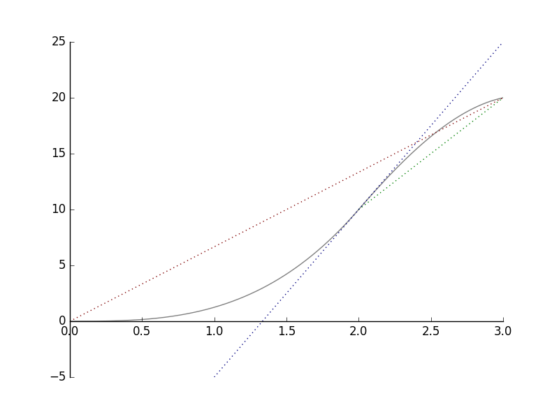
a) Look at the red line. We can see that in three hours, the cyclist moved \(20\)km. The average speed of the whole trip is \(6.6\) km/h.
b) Now look at the green line. We can see that during the third hour the cyclist moved \(10\)km further. That makes the average speed of that time interval \(10\) km/h.
Notice that the slope of the red line is \(20/3 \approx 6.6\) and that the slope of the blue line is \(10\). These are the same values as the corresponding average speeds.
c) Look at the blue line. It is the tangent of the curve at the point \(x=2h\). Using the same principle as with average speeds, we conclude that after two hours of the departure, the speed of the cyclist was \(30/2\) km/h \(= 15\) km/h.
Now we will proceed to the general definition:
Definition: Derivative
Let \((a,b)\subset \mathbb{R}\). The derivative of function \(f\colon (a,b)\to \mathbb{R}\) at the point \(x_0\in (a,b)\) is \[f'(x_0):=\lim_{h\to 0} \frac{f(x_0+h)-f(x_0)}{h}.\] If \(f'(x_0)\) exists, then \(f\) is said to be differentiable at the point \(x_0\).
Note: Since \(x = x_0+h\), then \(h=x-x_0\), and thus the definition can also be written in the form \[f'(x_0):=\lim_{x\to x_0} \frac{f(x)-f(x_0)}{x-x_0}.\]
The derivative can be denoted in different ways: \[ f'(x_0)=Df(x_0) =\left. \frac{df}{dx}\right|_{x=x_0}, \ \ f'=Df =\frac{df}{dx}. \]
Interpretation. Consider the curve \(y = f(x)\). Now if we draw a line through the points \((x_0,f(x_0))\) and \((x_0+h, f(x_0+h))\), we see that the slope of this line is \[\frac{f(x_0+h)-f(x_0)}{x_0+h-x_0} = \frac{f(x_0+h)-f(x_0)}{h}.\] When \(h \to 0\), the line intersects with the curve \(y = f(x)\) only in the point \((x_0, f(x_0))\). This line is the tangent of the curve \(y=f(x)\) at the point \((x_0,f(x_0))\) and its slope is \[\lim_{h\to 0} \frac{f(x_0+h)-f(x_0)}{h},\] which is the derivative of the function \(f\) at \( x_0\). Hence, the tangent is given by the equation \[y=f(x_0)+f'(x_0)(x-x_0).\]
Interactivity. Move the point of intersection and observe changes on the tangent line of the curve.
Example 1.
Let \(f\colon \mathbb{R} \to \mathbb{R}\) be the function \(f(x) = x^3 + 1\). The derivative of \(f\) at \(x_0 = 1\) is \[\begin{aligned}f'(1) &=\lim_{h \to 0} \frac{f(1+h)-f(1)}{h} \\ &=\lim_{h \to 0} \frac{(1+h)^3 + 1 - 1^3 - 1}{h} \\ &=\lim_{h \to 0} \frac{1+3h+3h^2+h^3-1}{h} \\ &=\lim_{h \to 0} \frac{h(3+3h+h^2)}{h} \\ &=\lim_{h \to 0} 3+3h+h^2 \\ &= 3. \end{aligned}\]
Function \( x^3 + 1\) and its tangent at the point \(1\).
Example 2.
Let \(f\colon \mathbb{R} \to \mathbb{R}\) be the function \(f(x)=ax+b\). We find the derivative of \(f(x)\).
Immediately from the definition we get: \[\begin{aligned}f'(x) &=\lim_{h\to 0} \frac{f(x+h)-f(x)}{h} \\ &=\lim_{h\to 0} \frac{[a(x+h)+b]-[ax+b]}{h} \\ &=\lim_{h\to 0} a \\ &=a.\end{aligned}\]
Here \(a\) is the slope of the tangent line. Note that the derivative at \(x\) does not depend on \(x\) because \(y=ax+b\) is the equation of a line.
Note. When \(a=0\), we get \(f(x) = b\) and \(f'(x) = 0\). The derivative of a constant function is zero.
Example 3.
Let \(g\colon \mathbb{R} \to \mathbb{R}\) be the function \(g(x)=|x|\). Does \(g\) have a derivative at \(0\)?
Now \[g'(x_0)= \begin{cases}+1 & \text{when $x_{0}>0$} \\ -1 & \text{when $x_{0}<0$}\end{cases}\]
The graph \(y=g(x)\) has no tangent at the point \(x_0=0\): \[\frac{g(0+h)-g(0)}{h}= \frac{|0+h|-|0|}{h}=\frac{|h|}{h}=\begin{cases}+1 & \text{for $h>0$}, \\ -1 & \text{for $h<0$}.\end{cases}\] Thus \(g'(0)\) does not exist.
Conclusion. The function \(g\) is not differentiable at the point \(0\).
Remark. Let \(f\colon (a,b)\to \mathbb{R}\). If \(f'(x)\) exists for every \(x\in (a,b)\) then we get a function \(f'\colon (a,b)\to \mathbb{R}\). We write:
| (1) | \(f(x)\) | = \(f^{(0)}(x)\), | |
| (2) | \(f'(x)\) | = \(f^{(1)}(x)\) | = \(\frac{d}{dx}f(x)\), |
| (3) | \(f''(x)\) | = \(f^{(2)}(x)\) | = \(\frac{d^2}{dx^2}f(x)\), |
| (4) | \(f'''(x)\) | = \(f^{(3)}(x)\) | = \(\frac{d^3}{dx^3}f(x)\), |
| ... |
Here \(f''(x)\) is called the second derivative of \(f\) at \(x\), \(f^{(3)}\) is the third derivative, and so on.
We introduce the notation \begin{eqnarray} C^n\bigl( ]a,b[\bigr) =\{ f\colon \, ]a,b[\, \to \mathbb{R} & \mid & f \text{ is } n \text{ times differentiable on the interval } ]a,b[ \nonumber \\ & & \text{ and } f^{(n)} \text{ is continuous}\}. \nonumber \end{eqnarray} These functions are said to be n times continuously differentiable.
Function \(|x|\).
Example 4.
The distance moved by a cyclist (or a car) is given by \(s(t)\). Then the speed at the moment \(t\) is \(s'(t)\) and the acceleration is \(s''(t)\).
Linearization and differential
Properties of derivative
Next we give some useful properties of the derivative. These properties allow us to find derivatives for some familiar classes of functions such as polynomials and rational functions.
Continuity and derivative
If \(f\) is differentiable at the point \(x_0\), then \(f\) is continuous at the point \(x_0\): \[ \lim_{h\to 0} f(x_0+h) = f(x_0).\] Why? Because if \(f\) is differentiable, then we get \[f(x_0)+h\frac{f(x_0+h)-f(x_0)}{h} \rightarrow f(x_0)+0\cdot f'(x_0)=f(x_0),\] as \(h \to 0\).
Note. If a function is continuous at the point \(x_0\), it doesn't have to be differentiable at that point. For example, the function \(g(x) = |x|\) is continuous, but not differentiable at the point \(0\).
Differentiation Rules
Next we will give some important rules which are often applied in practical problems concerning determination of the derivative of a given function.
Suppose that \(f\) and \(g\) are differentiable at \(x\).
A Constant Multiplier
\[(cf)'(x) = cf'(x),\ c \in \mathbb{R}\]
Suppose that \(f\) is differentiable at \(x\). We determine: \[(cf)'(x),\] where \(c\in \mathbb{R}\) is a constant.
\[\begin{aligned}\frac{(cf)(x+h)-(cf)(x)}{h} \ & \ = \ \frac{cf(x+h)-cf(x)}{h} \\ & \ = \ c \ \frac{f(x+h)-f(x)}{h}\end{aligned}\]
As \(h\to 0\), we get \[c \ \frac{f(x+h)-f(x)}{h} \to c f'(x).\]
\(\square\)
The Sum Rule
\[(f+g)'(x) = f'(x) + g'(x)\]
Suppose that \(f\) and \(g\) are differentiable at \(x\). We determine \[(f+g)'(x).\]
By the definition: \[\begin{aligned}\frac{(f+g)(x+h)-(f+g)(x)}{h} \ & \ = \ \frac{[f(x+h)+g(x+h)]-[f(x)+g(x)]}{h} \\ & \ = \ \frac{f(x+h)-f(x)}{h}+\frac{g(x+h)-g(x)}{h}\end{aligned}\]
When \(h\to 0\), we get \[\frac{f(x+h)-f(x)}{h}+\frac{g(x+h)-g(x)}{h}\to \ f'(x)+g'(x)\]
\(\square\)
The Product Rule
\[(fg)'(x) = f'(x)g(x) + f(x)g'(x)\]
Suppose that \(f,g\) and are differentiable at \(x\). We determine \[(fg)'(x).\] \[\begin{aligned}\frac{(fg)(x+h)-(fg)(x)}{h} & = \frac{f(x+h)g(x+h)-f(x)g(x)}{h} \\ & = \frac{f(x+h)g(x+h)-f(x)g(x+h)+f(x)g(x+h)-f(x)g(x)}{h} \\ & = \frac{f(x+h)-f(x)}{h}\ g(x+h)+f(x)\ \frac{g(x+h)-g(x)}{h}\end{aligned}\]
When \(h\to 0\), we get \[\frac{f(x+h)-f(x)}{h}g(x+h)+f(x)\frac{g(x+h)-g(x)}{h}\to f'(x)g(x)+f(x)g'(x).\]
\(\square\)
The Power Rule
\[\frac{d}{dx} x^n = nx^{n-1} \text{, } n \in \mathbb{Z}\]
For \( n\ge 1\) we repeteadly apply the product rule, and obtain \[\begin{aligned}\frac{d}{dx}x^n \ & = \frac{d}{dx}(x\cdot x^{n-1}) \\ & = (\frac{d}{dx}x)x^{n-1}+x\frac{d}{dx}x^{n-1} \\ & \stackrel{dx/dx=1}{=} x^{n-1}+x\frac{d}{dx}x^{n-1} \\ & = x^{n-1}+x\left( x^{n-2}+x\frac{d}{dx}x^{n-2}\right) \\ & = \ldots \\ & = \sum_{k=0}^{n-1} x^{n-1} \\ & = nx^{n-1}.\end{aligned}\]
The case of negative \( n\) is obtained from this and the product rule applied to the identity \( x^n \cdot x^{-n} = 1\).
From the power rule we obtain a formula for the derivative of a polynomial. Let \[P(x)=a_n x^{n}+a_{n-1}x^{n-1}+\ldots+ a_1 x + a_0,\] where \(n\in \mathbb{N}\). Then \[\frac{d}{dx}P(x)=na_nx^{n-1}+(n-1)a_{n-1}x^{n-2}+\ldots +2 a_2 x+a_1.\]
\(\square\)
The Reciprocal Rule
\[\Big(\frac{1}{f}\Big)'(x) = - \frac{f'(x)}{f(x)^2} \text{, } f(x) \neq 0\]
Suppose that \(f\) is differentiable at \(x\) and \(f(x)\neq 0\). We determine \[(\frac{1}{f})'(x).\]
From the definition we obtain: \[\begin{aligned}\frac{(1/f)(x+h)-(1/f)(x)}{h} & = \frac{1/f(x+h)-1/f(x)}{h} \\ & = \frac{\frac{f(x)}{f(x)f(x+h)}-\frac{f(x+h)}{f(x)f(x+h)}}{h} \\ & = \frac{f(x)-f(x+h)}{h}\frac{1}{f(x)f(x+h)}\end{aligned}\]
Because \(f\) is differentiable at \(x\) we get \[\frac{f(x)-f(x+h)}{h}\frac{1}{f(x)f(x+h)}=-f'(x)/f(x)^2,\] as \(h\to 0\).
\(\square\)
The Quotient Rule
\[(f/g)'(x) = \frac{f'(x)g(x)-f(x)g'(x)}{g(x)^2},\ g(x) \neq 0\]
Suppose that \(f,g\) are differentiable at \(x\) and \(g(x)\neq 0\). Then \[\begin{aligned}(f/g)'(x) & = \Big( f \cdot \frac{1}{g}\Big) '(x) \\ & = f'(x)\frac{1}{g(x)}-f(x)\frac{g'(x)}{g(x)^2} \\ & = \frac{f'(x)g(x)-f(x)g'(x)}{g(x)^2}.\end{aligned}\]
\(\square\)
Interactivity. Vary \(x\) and the constant multiplier and see the effect of constant multiplier rule in practice.
Example 1.
\[\frac{d}{dx}(x^{2006}+5x^3+42)=\frac{d}{dx}x^{2006}+5\frac{d}{dx}x^3+42\frac{d}{dx}1=2006x^{2005}+5\cdot 3x^2.\]
Example 2.
\[\begin{aligned}\frac{d}{dx} [(x^4-2)(2x+1)] &= \frac{d}{dx}(x^4-2) \cdot (2x+1) + (x^4-2) \cdot \frac{d}{dx}(2x + 1) \\ &= 4x^3(2x+1) + 2(x^4-2) \\ &= 8x^4+4x^3+2x^4-4 \\ &= 10x^4+4x^3-4.\end{aligned}\]
Note. We can check the answer by deriving it in another way: \[\frac{d}{dx} [(x^4-2)(2x+1)] = \frac{d}{dx} (2x^5 +x^4 -4x -2) = 10x^4 +4x^3 -4.\]
Function \( (x^4-2)(2x+1) \).
Example 3.
For \(x \neq 0\) we get \[\frac{d}{dx} \frac{3}{x^3} = 3 \cdot \frac{d}{dx} \frac{1}{x^3} = -3 \cdot \frac{\frac{d}{dx} x^3}{(x^3)^2} = -3 \cdot \frac{3x^2}{x^6}= - \frac{9}{x^4}.\]
Note. There is another way of solving the problem above by noticing that \(\frac{1}{x^3} = x^{-3}\) and differentiating it as a power: \[\frac{d}{dx} \ \frac{3}{x^3} = 3 \cdot \frac{d}{dx} x^{-3} = 3 \cdot (-3x^{-4})= - \frac{9}{x^4}\]
Example 4.
\[\begin{aligned}\frac{d}{dx} \frac{x^3}{1+x^2} & = \frac{(\frac{d}{dx}x^3)(1+x^2)-x^3\frac{d}{dx}(1+x^2)}{(1+x^2)^2} \\ & = \frac{3x^2(1+x^2)-x^3(2x)}{(1+x^2)^2} \\ & = \frac{3x^2+x^4}{(1+x^2)^2}.\end{aligned}\]
Function \(x^3 / (1+x^2)\).
Rolle's Theorem
If \(f\) is differentiable at a local extremum \(x_0\in \, ]a,b[\), then \(f'(x_0)=0\).
The one-sided limits of the difference quotient have different signs at a local extremum. For example, for a local maximum it holds that \begin{eqnarray} \frac{f(x_0+h)-f(x_0)}{h} = \frac{\text{negative} }{\text{positive}}&\le& 0, \text{ when } h>0, \nonumber \\ \frac{f(x_0+h)-f(x_0)}{h} = \frac{\text{negative}}{\text{negative}}&\ge& 0, \text{ when } h<0 \nonumber \end{eqnarray} and \(|h|\) is so small that \(f(x_0)\) is a maximum on the interval \([x_0-h,x_0+h]\).
L'Hospital's Rule
There are many different versions of this rule, but we present only the simplest one. Let us assume that \(f(x_0)=g(x_0)=0\) and the functions \(f,g\) are differentiable on some interval \(]x_0-\delta,x_0+\delta[\). If \[ \lim_{x\to x_0}\frac{f'(x)}{g'(x)} \] exists, then \[ \lim_{x\to x_0}\frac{f(x)}{g(x)}=\lim_{x\to x_0}\frac{f'(x)}{g'(x)}. \]
In the special case \(g'(x_0)\neq 0\) the proof is simple: \[ \frac{f(x)}{g(x)}=\frac{f(x)-f(x_0)}{g(x)-g(x_0)} = \frac{\bigl( f(x)-f(x_0)\bigr) /(x-x_0)}{\bigl( g(x)-g(x_0)\bigr) /(x-x_0)} \to \frac{f'(x_0)}{g'(x_0)}. \] In the general case we need the so-called generalized mean value theorem, which states that \[ \frac{f(x)}{g(x)} = \frac{f'(c)}{g'(c)} \] for some \(c\in \, ]x_0,x[\). Here we have the same point \(c\) both in the numerator and the denominator, so we do not even need the continuity of the derivatives!
Derivatives of Trigonometric Functions
In this section, we give differentiation formulas for trigonometric functions \(\sin\), \(\cos\) and \(\tan\).
Derivative of Sine
\[\sin'(t)=\cos(t)\]
Function \(\sin(x)\) and its derivative function \(\cos(x)\).
Derivative of Cosine
\[\cos'(t)= - \sin(t)\]
This follows in a similar way as the derivative of Sine, but more easily from the identity \(\cos(t)=\sin(\pi/2-t)\) and the Chain rule to be introduced in the following section.
\(\square\)
Function \(\cos(x)\) and its derivative function \(-\sin(x)\).
Derivative of Tangent
\[\tan'(t) = \frac{1}{\cos^2(t)}=1+\tan^2 t.\]
Because \[\tan(t)=\frac{\sin(t)}{\cos(t)},\] from the quotient rule we obtain \[\tan'(t)=\frac{\sin'(t)\cos(t)-\sin(t)\cos'(t)}{\cos^2(t)}=\frac{\cos^2(t)+\sin^2(t)}{\cos^2(t)}=\begin{cases}\frac{1}{\cos^2(t)} & \\ 1+\tan^2 t.\end{cases}\]
\(\square\)
Function \(\tan(x)\) and its derivative function \(1/\cos^2(x)\).
Example 1.
\[\frac{d}{dx} (3 \sin(x)) = 3 \sin'(x) = 3 \cos(x).\]
Example 2.
\[\frac{d}{dx} \cos^2 (x) = \cos'(x) \cdot \cos(x) + \cos(x) \cdot \cos'(x) = -2\sin(x)\cos(x).\]
Example 3.
\[\begin{aligned} \frac{d}{dx} \frac{\sin(x) + 1}{\cos(x)} &= \frac{d}{dx} \left( \frac{\sin(x)}{\cos(x)} + \frac{1}{\cos(x)} \right) \\ &= \tan'(x) - \frac{\cos'(x)}{\cos^2(x)} \\ &= \frac{1+\sin(x)}{\cos^2 (x)}.\end{aligned}\]
The Chain Rule
In this section we learn a formula for finding the derivative of a composite function. This important formula is known as the Chain Rule.
The Chain Rule.
Let \(f\colon \mathbb{R}\to \mathbb{R}\), \(g\colon \mathbb{R}\to \mathbb{R}\) and \(f \circ g \colon \mathbb{R}\to \mathbb{R}\).
Let \(g\) be differentiable at the point \(x\) and \(f\) at \(g(x)\). Then
\[\frac{d}{dx}f(g(x))=f'(g(x))g'(x).\]
Consider
\[\begin{aligned}\frac{f(g(x+h))-f(g(x))}{h} &= \frac{f(g(x+h))-f(g(x))}{h} \ \frac{g(x+h)-g(x)}{g(x+h)-g(x)} \\ &= \frac{f(g(x+h))-f(g(x))}{g(x+h)-g(x)} \ \frac{g(x+h)-g(x)}{h}.\end{aligned}\]
Now let us write \(k(h):=g(x+h)-g(x)\). Then \(g(x+h)=g(x)+k(h)\) and we get \[\frac{f(g(x+h))-f(g(x))}{h}=\frac{f(g(x)+k(h))-f(g(x))}{k(h)}\frac{g(x+h)-g(x)}{h}.\]
Problem. What if \(k(h)=0\)? Note that one cannot divide by zero.
Solution. Define \[E(k):= \begin{cases}0, & \text{for $k=0$}, \\ \frac{f(g(x)+k)-f(g(x))}{k}-f'(g(x)), & \text{for $k\neq 0$},\end{cases}\] so that \[\frac{f(g(x+h))-f(g(x))}{h}=[E(k(h))+f'(g(x))]\frac{g(x+h)-g(x)}{h}.\] Now, because \(E\) is continuous, we get \[[E(k(h))+f'(g(x))]\frac{g(x+h)-g(x)}{h}\to f'(g(x))g'(x).\] as \(h\to 0\).
\(\square\)
Example 1.
The problem is to differentiate the function \((2x-1)^3\). We take \(f(x) = x^3\) and \(g(x) = 2x-1\) and differentiate the composite function \(f(g(x))\). As \[f'(x) = 3x^2 \text{ and } g'(x) = 2,\] we get \[\frac{d}{dx} (2x-1)^3 = 3(2x-1)^2 \cdot 2 = 6(4x^2-4x+1) = 24x^2-24x+6.\]
Function \((2x-1)^3\) and its derivative function.
Example 2.
We need to differentiate the function \(\sin 3x\). Take \(f(x) = \sin x\) and \(g(x) = 3x\), then differentiate the composite function \(f(g(x))\). \[\frac{d}{dx} \sin 3x = \cos 3x \cdot 3 = 3 \cos 3x.\]
Remark. Let \(h\colon \mathbb{R}\to \mathbb{R}, g\colon \mathbb{R}\to \mathbb{R}\) and \(f\colon \mathbb{R}\to \mathbb{R}\). Now \[\frac{d}{dx}f(g(h(x)))=f'(g(h(x)))\frac{d}{dx}g(h(x))=f'(g(h(x)))g'(h(x))h'(x).\] Similarly, one may obtain even more complex rules for composites of multiple functions.
Function \(\sin 3x\) and its derivative function.
Example 3.
Differentiate the function \(\cos^3 2x\). Take \(f(x) = x^3\), \(g(x) = \cos x\) and \(h(x) = 2x\) and differentiate the composite function \(f(g(h(x)))\). \[\begin{aligned}\frac{d}{dx} \cos^3 2x &= 3(\cos 2x)^2 \cdot \frac{d}{dx} \cos 2x \\ &= 3 \cos^2 2x \cdot (-\sin 2x) \cdot 2 \\ &= -6 \sin 2x \cos^2 2x.\end{aligned}\]
Function \(\cos^3 2x\) and its derivative function.
Extremal Value Problems
We will discuss the Intermediate Value Theorem for differentiable functions, and its connections to extremal value problems.
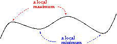
Definition: Local Maxima and Minima
A function \(f\colon A\to \mathbb{R}\) has a a local maximum at the point \(x_0\in A\), if for some \(h\gt 0\) and for all \(x\in A\) such that \(|x-x_0|\lt h\), we have \(f(x)\leq f(x_0)\).
Similarly, a function \(f\colon A\to \mathbb{R}\) has a local minimum at the point \(x_0\in A\) , if for some \(h>0\) and for all \(x\in A\) such that \(|x-x_0|\lt h\), we have \(f(x)\geq f(x_0)\).
A local extreme is a local maximum or a local minimum.
Remark. If \(x_0\) is a local maximum value and \(f'(x_0)\) exists, then \[\begin{cases}f'(x_0) & =\lim_{h\to 0^{+}}\frac{f(x_0+h)-f(x_0)}{h} \leq 0 \\ f'(x_0) & =\lim_{h\to 0^{-}}\frac{f(x_0+h)-f(x_0)}{h} \geq 0.\end{cases}\] Hence \(f'(x_0)=0\).
We get:
Theorem 1.
Let \(x_0\in [a,b]\) be a local extremal value of a continuous function \(f\colon [a,b]\to \mathbb{R}\). Then either
the derivative \(f'(x_0)\) doesn't exist (this includes also cases \(x_0=a\) and \(x_0=b\)) or
\(f'(x_0)=0\).
Example 1.
Let \(f: \mathbb{R} \to \mathbb{R}\) be defined by \[f(x) = x^3 -3x + 1.\] Then \[f'(x) = 3x^2-3\] and we can see that at the points \(x_0 = -1\) and \(x_0 = 1\) the local maximum and minimum of \(f\) are obtained, \[f'(-1) = 3 \cdot (-1)^2 - 3 = 0 \text{ and } f'(1) = 3 \cdot 1^2 - 3 = 0.\]
Function \(x^3-3x+1\) and its derivative function \(3x^2-3\).
Finding the global extrema
In practice, when we are looking for the local extrema of a given function, we need to check three kinds of points:
the zeros of the derivative
the endpoints of the domain of definition (interval)
points where the function is not differentiable
If we happened to know beforehand that the function has a minimum/maximum, then we start off by finding all the possible local extrema (the points described above), evaluate the function at these points and pick the greatest/smallest of these values.
Example 2.
Let us find the smallest and greatest value of the function \(f\colon [0,2]\to \mathbf{R}\), \(f(x)=x^3-6x\). Since the function is continuous on a closed interval, then it has a maximum and a minimum. Since the function is differentiable, it is sufficient to examine the endpoints of the interval and the zeros of the derivative that are contained in the interval.
The zeros of the derivative: \(f'(x)=3x^2-6=0 \Leftrightarrow x=\pm \sqrt{2}\). Since \(-\sqrt{2}\not\in [0,2]\), we only need to evaluate the function at three points, \(f(0)=0\), \(f(\sqrt{2})=-4\sqrt{2}\) and \(f(2)=-4\). From these we can see that the smallest value of the function is \(-4\sqrt{2}\) and the greatest value is \(0\), respectively.
Next we will formulate a fundamental result for differentiable functions. The basic idea here is that the change on an interval can only happen, if there is change at some point on the inverval.
Theorem 2.
(The Intermediate Value Theorem for Differentiable Functions). Let \(f\colon [a,b]\to \mathbb{R}\) be continuous in the interval \([a,b]\) and differentiable in the interval \((a,b)\). Then \[f'(x_0)=\frac{f(b)-f(a)}{b-a}\] for some \(x_0\in (a,b).\)
Let \(f\) be continuous in the interval \([a,b]\) and differentiable in the interval \((a,b)\). Let us define \[g(x):=f(x)-\frac{f(b)-f(a)}{b-a}(x-a)-f(a).\]
Now \(g(a)=g(b)=0\) and \(g\) is differentiable in the interval \((a,b)\). According to Rolle's Theorem, there exists \(c\in(a,b)\) such that \(g'(c)=0\). Hence \[f'(c)=g'(c)+\frac{f(b)-f(a)}{b-a}=\frac{f(b)-f(a)}{b-a}.\]
\(\square\)
This result has an important application:
Theorem 3.
Let \(f\colon (a,b)\to \mathbb{R}\) be a differentiable function. Then
If for all \(x\in (a,b) \ \ f'(x)\geq 0\), then \(f\) is increasing,
If for all \(x\in (a,b) \ \ f'(x)\leq 0\), then \(f\) is decreasing.
Suppose that \(a \lt x_1 \lt x_2 \lt b\).
Then by Theorem 2 there exists \(x_0\in (x_1,x_2)\) such that \[f'(x_0)=\frac{f(x_2)-f(x_1)}{x_2-x_1}.\]
It follows that \(f(x_2)-f(x_1)=f'(x_0)(x_2-x_1)\).
Hence we may conclude that \(f\) is increasing for \(f'(x_0)\geq 0\) and decreasing for \(f'(x_0)\leq 0\).
Example 3.
For the polynomial \(f(x) = \frac{1}{4} x^4-2x^2-7\) the derivative is \[f'(x) = x^3-4x = x(x^2-4) = 0,\] when \(x=0\), \(x=2\) or \(x=-2\). Now we can draw a table:
| \(x<-2\) | \(-2 \lt x \lt 0\) | \(0 \lt x \lt 2\) | \(x>2\) | |
|---|---|---|---|---|
| \(x\) | \(<0\) | \(<0\) | \(>0\) | \(>0\) |
| \(x^2-4\) | \(>0\) | \(<0\) | \(<0\) | \(>0\) |
| \(f'(x)\) | \(<0\) | \(>0\) | \(<0\) | \(>0\) |
| \(f(x)\) | decr. | incr. | decr. | incr. |
Function \(\frac{1}{4} x^4-2x^2-7\).
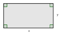
Example 4.
We need to find a rectangle so that its area is \(9\) and it has the least possible perimeter.
Let \(x\ (>0)\) and \(y\ (>0)\) be the sides of the rectangle. Then \(x \cdot y = 9\) and we get \(y=\frac{9}{x}\). Now the perimeter is \[2x+2y = 2x+2 \frac{9}{x} = \frac{2x^2+18}{x}.\] In which point does the function \(f(x) = \frac{2x^2+18}{x}\) get its minimum value? Function \(f\) is continuous and differentiable, when \(x>0\) and using the quotient rule, we get \[f'(x) = \frac{4x \cdot x-(2x^2+18) \cdot 1}{x^2} = \frac{2x^2-18}{x^2}.\] Now \(f'(x) = 0\), when \[\begin{aligned}2x^2-18 &= 0 \\ 2x^2 &= 18 \\ x^2 &= 9 \\ x &= \pm 3\end{aligned}\] but we have defined that \(x>0\) and therefore are only interested in the case \(x=3\). Let's draw a table:
| \(x<3\) | \(x>3\) | |
|---|---|---|
| \(f'(x)\) | \(<0\) | \(>0\) |
| \(f(x)\) | decr. | incr. |
As the function \(f\) is continuous, we now know that it attains its minimum at the point \(x=3\). Now we calculate the other side of the rectangle: \(y=\frac{9}{x}=\frac{9}{3}=3\).
Thus, the rectangle, which has the least possible perimeter is actually a square, which sides are of the length \(3\).
Function \(\frac{2x^2+18}{x}\).
Example 5.
We must make a one litre measure, which is shaped as a right circular cylinder without a lid. The problem is to find the best size of the bottom and the height so that we need the least possible amount of material to make the measure.
Let \(r > 0\) be the radius and \(h > 0\) the height of the cylinder. The volume of the cylinder is \(1\) dm\(^3\) and we can write \(\pi r^2 h = 1\) from which we get \[h = \frac{1}{\pi r^2}.\]
The amount of material needed is the surface area \[A_{\text{bottom}} + A_{\text{side}} = \pi r^2 + 2 \pi r h = \pi r^2 + \frac{2 \pi r}{\pi r^2} = \pi r^2 + \frac{2}{r}.\]
Let function \(f: (0, \infty) \to \mathbb{R}\) be defined by \[f(r) = \pi r^2 + \frac{2}{r}.\] We must find the minimum value for function \(f\), which is continuous and differentiable, when \(r>0\). Using the reciprocal rule, we get \[f'(r) = 2\pi r -2 \cdot \frac{1}{r^2} = \frac{2\pi r^3 - 2}{r^2}.\] Now \(f'(r) = 0\), when \[\begin{aligned}2\pi r^3 - 2 &= 0 \\ 2\pi r^3 &= 2 \\ r^3 &= \frac{1}{\pi} \\ r &= \frac{1}{\sqrt[3]{\pi}}.\end{aligned}\]
Let's draw a table:
| \(r<\frac{1}{\sqrt[3]{\pi}}\) | \(r>\frac{1}{\sqrt[3]{\pi}}\) | |
|---|---|---|
| \(f'(r)\) | \(<0\) | \(>0\) |
| \(f(r)\) | decr. | incr. |
As the function \(f\) is continuous, we now know that it gets its minimum value at the point \(r= \frac{1}{\sqrt[3]{\pi}} \approx 0.683\). Then \[h = \frac{1}{\pi r^2} = \frac{1}{\pi \left(\frac{1}{\sqrt[3]{\pi}}\right)^2} = \frac{1}{\frac{\pi}{\pi^{2/3}}} = \frac{1}{\sqrt[3]{\pi}} \approx 0.683.\]
This means that it would take least materials to make a measure, which is approximately \(2 \cdot 0.683\) dm \( = 1.366\) dm \( \approx 13.7\) cm in diameter and \(0.683\) dm \( \approx 6.8\) cm high.

Function \(\pi r^2 + \frac{2}{r}\).
5. Taylor polynomial
Taylor polynomial
Example
Compare the graph of \(\sin x\) (red) with the graphs of the polynomials \[ x-\frac{x^3}{3!}+\frac{x^5}{5!}-\dots + \frac{(-1)^nx^{2n+1}}{(2n+1)!} \] (blue) for \(n=1,2,3,\dots,12\).
\(\displaystyle\sum_{k=0}^{n}\frac{(-1)^{k}x^{2k+1}}{(2k+1)!}\)
Definition: Taylor polynomial
Let \(f\) be \(k\) times differentiable at the point \(x_{0}\). Then the Taylor polynomial \begin{align} P_n(x)&=P_n(x;x_0)\\\ &=f(x_0)+f'(x_0)(x-x_0)+\frac{f''(x_0)}{2!}(x-x_0)^2+ \\ & \dots +\frac{f^{(n)}(x_0)}{n!}(x-x_0)^n\\ &=\sum_{k=0}^n\frac{f^{(k)}(x_0)}{k!}(x-x_0)^k\\ \end{align} is the best polynomial approximation of degree \(n\) (with respect to the derivative) for a function \(f\), close to the point \(x_0\).
Note. The special case \(x_0=0\) is often called the Maclaurin polynomial.
If \(f\) is \(n\) times differentiable at \(x_0\), then the Taylor polynomial has the same derivatives at \(x_0\) as the function \(f\), up to the order \(n\) (of the derivative).
The reason (case \(x_0=0\)): Let \[ P_n(x)=c_0+c_1x+c_2x^2+c_3x^3+\dots +c_nx^n, \] so that \begin{align} P_n'(x)&=c_1+2c_2x+3c_3x^2+\dots +nc_nx^{n-1}, \\ P_n''(x)&=2c_2+3\cdot 2 c_3x\dots +n(n-1)c_nx^{n-2} \\ P_n'''(x)&=3\cdot 2 c_3\dots +n(n-1)(n-2)c_nx^{n-3} \\ \dots && \\ P^{(k)}(x)&=k!c_k + x\text{ terms} \\ \dots & \\ P^{(n)}(x)&=n!c_n \\ P^{(n+1)}(x)&=0. \end{align}
From these way we obtain the coefficients one by one: \begin{align} c_0= P_n(0)=f(0) &\Rightarrow c_0=f(0) \\ c_1=P_n'(0)=f'(0) &\Rightarrow c_1=f'(0) \\ 2c_2=P_n''(0)=f''(0) &\Rightarrow c_2=\frac{1}{2}f''(0) \\ \vdots & \\ k!c_k=P_n^{(k)}(0)=f^{(k)}(0) &\Rightarrow c_k=\frac{1}{k!}f^{(k)}(0). \\ \vdots &\\ n!c_n=P_n^{(n)}(0)=f^{(n)}(0) &\Rightarrow c_k=\frac{1}{n!}f^{(n)}(0). \end{align} Starting from index \(k=n+1\) we cannot pose any new conditions, since \(P^{(n+1)}(x)=0\).
Taylor's Formula
If the derivative \(f^{(n+1)}\) exists and is continuous on some interval \(I=\, ]x_0-\delta,x_0+\delta[\), then \(f(x)=P_n(x;x_0)+E_n(x)\) and the error term \(E_n(x)\) satisfies \[ E_n(x)=\frac{f^{(n+1)}(c)}{(n+1)!}(x-x_0)^{n+1} \] at some point \(c\in [x_0,x]\subset I\). If there is a constant \(M\) (independent of \(n\)) such that \(|f^{(n+1)}(x)|\le M\) for all \(x\in I\), then \[ |E_n(x)|\le \frac{M}{(n+1)!}|x-x_0|^{n+1} \to 0 \] as \(n\to\infty\).
\neq omitted here (mathematical induction or integral).
Examples of Maclaurin polynomial approximations: \begin{align} \frac{1}{1-x} &\approx 1+x+x^2+\dots +x^n =\sum_{k=0}^{n}x^k\\ e^x&\approx 1+x+\frac{1}{2!}x^2+\frac{1}{3!}x^3+\dots + \frac{1}{n!}x^n =\sum_{k=0}^{n}\frac{x^k}{k!}\\ \ln (1+x)&\approx x-\frac{1}{2}x^2+\frac{1}{3}x^3-\dots + \frac{(-1)^{n-1}}{n}x^n =\sum_{k=1}^{n}\frac{(-1)^{k-1}}{k}x^k\\ \sin x &\approx x-\frac{1}{3!}x^3+\frac{1}{5!}x^5-\dots +\frac{(-1)^n}{(2n+1)!}x^{2n+1} =\sum_{k=0}^{n}\frac{(-1)^k}{(2k+1)!}x^{2k+1}\\ \cos x &\approx 1-\frac{1}{2!}x^2+\frac{1}{4!}x^4-\dots +\frac{(-1)^n}{(2n)!}x^{2n} =\sum_{k=0}^{n}\frac{(-1)^k}{(2k)!}x^{2k} \end{align}
Example
Which polynomial \(P_n(x)\) approximates the function \(\sin x\) in the interval \([-\pi,\pi]\) so that the absolute value of the error is less than \(10^{-6}\)?
We use Taylor's Formula for \(f(x)=\sin x\) at \(x_0=0\). Then \(|f^{(n+1)}(c)|\le 1\) independently of \(n\) and the point \(c\). Also, in the interval in question, we have \(|x-x_0|=|x|\le \pi\). The requirement will be satisfied (at least) if \[ |E_n(x)|\le \frac{1}{(n+1)!}\pi^{n+1} < 10^{-6}. \] This inequality must be solved by trying different values of \(n\); it is true for \(n\ge 16\).
The required approximation is achieved with \(P_{16}(x)\), which fo sine is the same as \(P_{15}(x)\).
Check from graphs: \(P_{13}(x)\) is not enough, so the theoretical bound is sharp!
Taylor polynomial and extreme values
If \(f'(x_0)=0\), then also some higher derivatives may be zero: \[ f'(x_0)=f''(x_0)= \dots = f^{(n)}(x_0) =0,\ f^{(n+1)}(x_0) \neq 0. \] Then the behaviour of \(f\) near \(x=x_0\) is determined by the leading term (after the constant term \(f(x_0)\)) \[ \frac{f^{(n+1)}(x_0)}{(n+1)!}(x-x_0)^{n+1}. \] of the Taylor polynomial.
This leads to the following result:
Extreme values
- If \(n\) is even, then \(x_0\) is not an extreme point of \(f\).
- If \(n\) is odd and \(f^{(n+1)}(x_0)>0\), then \(f\) has a local minimum at \(x_0\).
- If \(n\) is odd and \(f^{(n+1)}(x_0)<0\), then \(f\) has a local maximum at \(x_0\).
Newton's method
The first Taylor polynomial \(P_1(x)=f(x_0)+f'(x_0)(x-x_0)\) is the same as the linearization of \(f\) at the point \(x_0\). This can be used in some simple approximations and numerical methods.
Newton's method
The equation \(f(x)=0\) can be solved approximately by choosing a starting point \(x_0\) (e.g. by looking at the graph) and defining \[ x_{n+1}=x_n-\frac{f(x_n)}{f'(x_n)} \] for \(n=0,1,2,\dots\) This leads to a sequence \((x_0,x_1,x_2,\dots )\), whose terms usually give better and better approximations for a zero of \(f\).
The recursion formula is based on the geometric idea of finding an approximative zero of \(f\) by using its linearization (i.e. the tangent line).
Example
Find an approximate value of \(\sqrt{2}\) by using Newton's method.
We use Newton's method for the function \(f(x)=x^2-2\) and initial value \(x_0=2\). The recursion formula becomes \[ x_{n+1}= x_n-\frac{x_n^2-2}{2x_n} = \frac{1}{2}\left(x_n+\frac{2}{x_n}\right), \] from which we obtain \(x_1=1{,}5\), \(x_2\approx 1{,}41667\), \(x_3\approx 1{,}4142157\) and so on.
By experimenting with these values, we find that the number of correct decimal places doubles at each step, and \(x_7\) gives already 100 correct decimal places, if intermediate steps are calculated with enough precision.
Taylor series
Taylor series
If the error term \(E_n(x)\) in Taylor's Formula goes to zero as \(n\) increases, then the limit of the Taylor polynomial is the Taylor series of \(f\) (= Maclaurin series for \(x_0=0\)).
The Taylor series of \(f\) is of the form \[ \sum_{k=0}^{\infty}\frac{f^{(k)}(x_0)}{k!}(x-x_0)^k = \lim_{n\to\infty} \sum_{k=0}^{n}\frac{f^{(k)}(x_0)}{k!}(x-x_0)^k . \] This is an example of a power series.
The Taylor series can be formed as soon as \(f\) has derivatives of all orders at \(x_0\) and they are substituted into this formula. There are two problems related to this: Does the Taylor series converge for all values of \(x\)?
Answer: Not always; for example, the function \[ f(x)=\frac{1}{1-x} \] has a Maclaurin series (= geometric series) converging only for \(-1 < x < 1\), although the function is differentiable for all \(x\neq 1\): \[ f(x)=\frac{1}{1-x} = 1+x+x^2+x^3+x^4+\dots \]
If the series converges for some \(x\), then does its sum equal \(f(x)\)? Answer: Not always; for example, the function \[ f(x)=\begin{cases} e^{-1/x^2}, & x\neq 0,\\ 0, & x=0,\\ \end{cases} \] satisfies \(f^{(k)}(0)=0\) for all \(k\in \mathbf{N}\) (elementary but difficult calculation). Thus its Maclaurin series is identically zero and converges to \(f(x)\) only at \(x=0\).
Conclusion: Taylor series should be studied carefully using the error terms. In practice, the series are formed by using some well known basic series.
Examples
\begin{align} \frac{1}{1-x} &= \sum_{k=0}^{\infty} x^k,\ \ |x|< 1 \\ e^x &= \sum_{k=0}^{\infty} \frac{1}{k!}x^k, \ \ x\in \mathbb{R} \\ \sin x &= \sum_{k=0}^{\infty} \frac{(-1)^{k}}{(2k+1)!} x^{2k+1}, \ \ x\in \mathbb{R} \\ \cos x &= \sum_{k=0}^{\infty} \frac{(-1)^{k}}{(2k)!} x^{2k},\ \ x\in \mathbb{R} \\ (1+x)^r &= 1+\sum_{k=1}^{\infty} \frac{r(r-1)(r-2)\dots (r-k+1)}{k!}x^k, |x|<1 \end{align} The last is called the Binomial Series and is valid for all \(r\in \mathbb{R}\). If \(r=n \in \mathbb{N}\), then starting from \(k=n+1\), all the coefficients are zero and in the beginning \[ \binom{n}{k} =\frac{n!}{k!(n-k)!} = \frac{n(n-1)(n-2)\dots (n-k+1)}{k!}. \]
Compare this to the Binomial Theorem: \[ (a+b)^n=\sum_{k=0}^n\binom{n}{k} a^{n-k}b^k =a^n +na^{n-1}b+\dots +b^n \] for \(n\in\mathbb{N}\).
Power series
Definition: Power series
A power series is of the form \[ \sum_{k=0}^{\infty} c_k(x-x_0)^k = \lim_{n\to\infty} \sum_{k=0}^{n}c_k(x-x_0)^k. \] The point \(x_0\) is the centre and the \(c_k\) are the coefficients of the series.
The series converges at \(x\) if the above limit is defined.
There are only three essentially different cases:
Abel's Theorem.
- The power series converges only for \(x=x_0\) (and then it consists of the constant \(c_0\) only)
- The power series converges for all \(x\in \mathbb{R}\)
- The power series converges on some interval \(]x_0-R,x_0+R[\) (and possibly in one or both of the end points), and diverges for other values of \(x\).
The number \(R\) is the radius of convergence of the series. In the first two cases we say that \(R=0\) or \(R=\infty\) respectively.
Example
For which values of the variable \(x\) does the power series \[\sum_{k=1}^{\infty} \frac{k}{2^k}x^k\] converge?
We use the ratio test with \(a_k=kx^k/2^k\). Then \[ \left| \frac{a_{k+1}}{a_k} \right| = \left| \frac{(k+1)x^{k+1}/2^{k+1}}{kx^k/2^k} \right| = \frac{k+1}{2k}|x| \to \frac{|x|}{2} \] as \(k\to\infty\). By the ratio test, the series converges for \(|x|/2<1\), and diverges for \(|x|/2>1\). In the border-line cases \(|x|/2= 1\Leftrightarrow x=\pm 2\) the general term of the series does not tend to zero, so the series diverges.
Result: The series converges for \(-2< x< 2\), and diverges otherwise.
Definition: Sum function
In the interval \(I\) where the series converges, we can define a function \(f\colon I\to \mathbb{R}\) by setting \begin{equation} \label{summafunktio} f(x) = \sum_{k=0}^{\infty} c_k(x-x_0)^k, \tag{1} \end{equation} which is called the sum function of the power series.
The sum function \(f\) is continuous and differentiable on \(]x_0-R,x_0+R[\). Moreover, the derivative \(f'(x)\) can be calculated by differentiating the sum function term by term: \[ f'(x)=\sum_{k=1}^{\infty}kc_k(x-x_0)^{k-1}. \] Note. The constant term \(c_0\) disappears and the series starts with \(k=1\). The differentiated series converges in the same interval \(x\in \, ]x_0-R,x_0+R[\); this may sound a bit surprising because of the extra coefficient \(k\).
Example
Find the sum function of the power series \(1+2x+3x^2+4x^3+\dots\)
This series is obtained by differentiating termwise the geometric series (with \(q=x\)). Therefore, \begin{align} 1+2x+3x^2+4x^3+\dots &= D(1+x+x^2+x^3+x^4+\dots ) \\ &= \frac{d}{dx}\left( \frac{1}{1-x}\right) = \frac{1}{(1-x)^2}. \end{align} Multiplying with \(x\) we obtain \[ \sum_{k=1}^{\infty}kx^{k} = x+2x^2+3x^3+4x^4+\dots = \frac{x}{(1-x)^2}, \] which is valid for \(|x|<1\).
In the case \([a,b]\subset\ ]x_0-R,x_0+R[\) we can also integrate the sum function termwise: \[ \int_a^b f(x)\, dx = \sum_{k=0}^{\infty}c_k\int_a^b (x-x_0)^k\, dx. \] Often the definite integral can be extended up to the end points of the interval of convergence, but this is not always the case.
Example
Calculate the sum of the alternating harmonic series.
Let us first substitute \(q=-x\) to the geometric series. This yields \[ 1-x+x^2-x^3+x^4-\dots =\frac{1}{1-(-x)} = \frac{1}{1+x}. \] By integrating both sides from \(x=0\) to \(x=1\) we obtain \[ 1-\frac{1}{2}+\frac{1}{3}-\frac{1}{4}+\dots =\int_0^1\frac{1}{1+x} =\ln 2. \] Note. Extending the limit of integration all the way up to \(x=1\) should be justified more rigorously here. We shall return to integration later on the course.
6. Elementary functions
This chapter gives some background to the concept of a function. We also consider some elementary functions from a (possibly) new viewpoint. Many of these should already be familiar from high school mathematics, so in some cases we just list the main properties.
Functions
Definition: Function
A function \(f\colon A\to B\) is a rule that determines for each element \(a\in A\) exactly one element \(b\in B\). We write \(b=f(a)\).
Definition: Domain and codomain
In the above definition of a function \(A=D_f\) is the domain (of definition) of the function \(f\) and \(B\) is called the codomain of \(f\).
Definition: Image of a function
The image of \(f\) is the subset
\(f[A]= \{ f(a) \mid a\in A\}\) of \(B\). An alternative name for image is range.
For example, \(f\colon \mathbb{R}\to\mathbb{R}\), \(f(x)=x^2\), has codomain \(\mathbb{R}\), but its image is \(f[\mathbb{R} ] =[0,\infty[\).
The function in the previous example can also be defined as \(f\colon \mathbb{R}\to [0,\infty[\), \(f(x)=x^2\), and then the codomain is the same as the image. In principle, this modification can always be done, but it is not reasonable in practice.
Example: Try to do the same for \(f\colon \mathbb{R}\to\mathbb{R}\), \(f(x)=x^6+x^2+x\), \(x\in\mathbb{R}\).
If the domain \(A\subset \mathbb{R}\) then \(f\) is a function of one (real) variable: the main object of study in this course.
If \(A\subset \mathbb{R}^n\), \(n\ge 2\), then \(f\) is a function of several variables (a multivariable function)
Inverse functions
Definition: Injection, surjection and bijection
A function \(f\colon A \to B\) is- injective (one-to-one) if it has different values at different points; i.e. \[x_1\neq x_2 \Rightarrow f(x_1)\neq f(x_2),\] or equivalently \[f(x_1)= f(x_2) \Rightarrow x_1=x_2.\]
- surjective (onto) if its image is the same as codomain, i.e. \(f[A]=B\)
- bijective (one-to-one and onto) if it is both injective and surjective.
Observe: A function becomes surjective if all redundant points of the codomain are left out. A function becomes injective if the domain is reduced so that no value of the function is obtained more than once.
Another way of defining these concepts is based on the number of solutions to an equation:
Definition
For a fixed \(y\in B\), the equation \(y=f(x)\) has
- at most one solution \(x\in A\) if \(f\) is injective
- at least one solution \(x\in A\) if \(f\) is surjective
- exactly one solution \(x\in A\) if \(f\) on bijective.
Definition: Inverse function
If \(f\colon A \to B\) is bijective, then it has an inverse \(f^{-1}\colon B \to A\), which is uniquely determined by the condition \[y=f(x) \Leftrightarrow x = f^{-1}(y).\]
The inverse satisfies \(f^{-1}(f(a))=a\) for all \(a\in A\) and \(f(f^{-1}(b))=b\) for all \(b\in B\).
The graph of the inverse is the mirror image of the graph of \(f\) with respect to the line \(y=x\): A point \((a,b)\) lies on the graph of \(f\) \(\Leftrightarrow\) \(b=f(a)\) \(\Leftrightarrow\) \(a=f^{-1}(b)\) \(\Leftrightarrow\) the point \((b,a)\) lies on the graph of \(f^{-1}\). The geometric interpretation of \((a,b)\mapsto (b,a)\) is precisely the reflection with respect to \(y=x\).
If \(A \subset \mathbb{R}\) and \(f\colon A\to \mathbb{R}\) is strictly monotone, then the function \(f\colon A \to f[A]\) has an inverse.
If here \(A\) is an interval and \(f\) is continuous, then also \(f^{-1}\) is is continuous in the set \(f[A]\).
Theorem: Derivative of the inverse
Let \(f\colon \, ]a,b[\, \to\, ]c,d[\) be differentiable and bijective, so that it has an inverse \(f^{-1}\colon \, ]c,d[\, \to\, ]a,b[\). As the graphs \(y=f(x)\) and \(y=f^{-1}(x)\) are mirror images of each other, it seems geometrically obvious that also \(f^{-1}\) is differentiable, and we actually have \[ \left(f^{-1}\right)'(x)=\frac{1}{f'(f^{-1}(x))}, \] if \(f'(f^{-1}(x))\neq 0\).
Differentiate both sides of the equation \begin{align} f(f^{-1}(x)) &= x \\ \Rightarrow f'(f^{-1}(x))\left(f^{-1}\right)'(x) &= Dx = 1, \end{align} and solve for \(\left(f^{-1}\right)'(x)\).
\(\square\)
Note. \(f'(f^{-1}(x))\) is the derivative of \(f\) at the point \(f^{-1}(x)\).
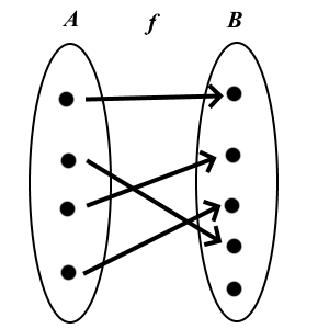
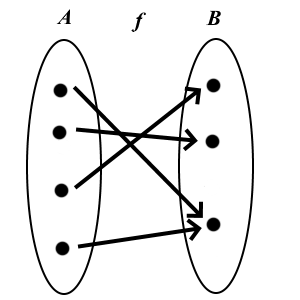
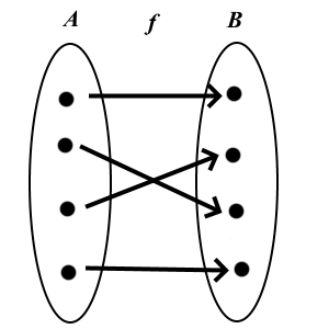
Transcendental functions
Trigonometric functions
Unit of measurement of an angle = rad: the arclength of the arc on the unit circle, that corresponds to the angle.
\(\pi\) rad = \(180\) degrees, i.e. \(1\) rad = \(180/\pi \approx 57,\! 3\) degrees
The functions \(\sin x, \cos x\) are defined in terms of the unit circle so that \((\cos x,\sin x)\), \(x\in [0,2\pi]\), is the point on the unit circle corresponding to the angle \(x\in\mathbb{R}\), measured counterclockwise from the point \((1,0)\). \[\tan x = \frac{\sin x}{\cos x}\ (x\neq \pi /2 +n\pi),\] \[\cot x = \frac{\cos x}{\sin x}\ (x\neq n\pi)\]
Periodicity: \[\sin (x+2\pi) = \sin x,\ \cos (x+2\pi)=\cos x,\] \[\tan (x+\pi) = \tan x\]
\(\sin 0 = 0\), \(\sin (\pi/2)=1\)
\(\cos 0=1\), \(\cos (\pi/2)= 0\)
Parity: \(\sin\) and \(\tan\) are odd functions, \(\cos\) is an even function: \[\sin (-x) = -\sin x,\] \[\cos(-x) = \cos x,\] \[\tan (-x) = -\tan x.\]
\(\sin^2 x + \cos^2 x = 1\) for all \(x\in\mathbb{R}\)
Proof: Pythagorean Theorem.
Addition formulas:
\(\sin (x+y) = \sin x \cos y +\cos x \sin y\)
\(\cos (x+y) = \cos x \cos y -\sin x \sin y\)
Basic properties (from the unit circle!)
Proof: Geometrically, or more easily with vectors and matrices.
Derivatives: \[ D(\sin x) = \cos x,\ \ D(\cos x) = -\sin x \]
Example
It follows that the functions \(y(t)=\sin (\omega t)\) and \(y(t)=\cos (\omega t)\) satisfy the differential equation \[ y''(t)+\omega^2y(t)=0, \] that models harmonic oscillation. Here \(t\) is the time variable and the constant \(\omega>0\) is the angular frequency of the oscillation. We will see later that all the solutions of this differential equation are of the form \[ y(t)=A\cos (\omega t) +B\sin (\omega t), \] with \(A,B\) constants. They will be uniquely determined if we know the initial location \(y(0)\) and the initial velocity \(y'(0)\). All solutions are periodic and their period is \(T=2\pi/\omega\).
where \(t\) is the elapsed time in seconds
Arcus functions
The trigonometric functions have inverses if their domain and codomains are chosen in a suitable way.
The Sine function \[ \sin \colon [-\pi/2,\pi/2]\to [-1,1] \] is strictly increasing and bijective.
The Cosine function \[ \cos \colon [0,\pi] \to [-1,1] \] is strictly decreasing and bijective.
The tangent function \[ \tan \colon ]-\pi/2,\pi/2[\, \to \mathbb{R} \] is strictly increasing and bijective.
Arcus functions
Inverses: \[\arctan \colon \mathbb{R}\to \ ]-\pi/2,\pi/2[,\] \[\arcsin \colon [-1,1]\to [-\pi/2,\pi/2],\] \[\arccos \colon [-1,1]\to [0,\pi]\]
This means: \[x = \tan \alpha \Leftrightarrow \alpha = \arctan x \ \ \text{for } \alpha \in \ ]-\pi/2,\pi/2[ \] \[x = \sin \alpha \Leftrightarrow \alpha = \arcsin x \ \ \text{for } \alpha \in \, [-\pi/2,\pi/2] \] \[x = \cos \alpha \Leftrightarrow \alpha = \arccos x \ \ \text{for } \alpha \in \, [0,\pi] \]
The graphs of \(\tan\) and \(\arctan\).
Derivatives of the arcus functions
\[D \arctan x = \frac{1}{1+x^2},\ x\in \mathbb{R} \tag{1}\] \[D\arcsin x = \frac{1}{\sqrt{1-x^2}},\ -1 < x < 1 \tag{2}\] \[D\arccos x = \frac{-1}{\sqrt{1-x^2}},\ -1 < x < 1 \tag{3}\]
Note. The first result is very useful in integration.
Here we will only prove the first result (1). By differentiating both sides of the equation \(\tan(\arctan x)=x\) for \(x\in \mathbb{R}\): \[\bigl( 1+\tan^2(\arctan x)\bigr) \cdot D(\arctan x) = D x = 1\] \[\Rightarrow D(\arctan x)= \frac{1}{1+\tan^2(\arctan x)}\] \[=\frac{1}{1+x^2}.\]
The last row follows also directly from the formula for the derivative of an inverse.
Example
Show that \[ \arcsin x +\arccos x =\frac{\pi}{2} \] for \(-1\le x\le 1\).
Example
Derive the addition formula for tan, and show that \[ \arctan x+\arctan y = \arctan \frac{x+y}{1+xy}. \]
Solutions: Voluntary exercises. The first can be deduced by looking at a rectangular triangle with the length of the hypotenuse equal to 1 and one leg of length \(x\).
Introduction: Radioactive decay
Let \(y(t)\) model the number of radioactive nuclei at time \(t\). During a short time interval \(\Delta t\) the number of decaying nuclei is (approximately) directly proportional to the length of the interval, and also to the number of nuclei at time \(t\): \[ \Delta y = y(t+\Delta t)-y(t) \approx -k\cdot y(t)\cdot \Delta t. \] The constant \(k\) depends on the substance and is called the decay constant. From this we obtain \[ \frac{\Delta y}{\Delta t} \approx -ky(t), \] and in the limit as \(\Delta t\to 0\) we end up with the differential equation \(y'(t)=-ky(t)\).
Exponential function
Definition: Euler's number
Euler's number (or Napier's constant) is defined as \[e = \lim_{n\to \infty} \left( 1+\frac{1}{n}\right) ^n = 1+1+\frac{1}{2!}+\frac{1}{3!} +\frac{1}{4!} +\dots \] \[\approx 2,\! 718281828459\dots\]
Definition: Exponential function
The Exponential function exp: \[ \exp (x) = \sum_{k=0}^{\infty} \frac{x^k}{k!}= \lim_{n\to \infty} \left( 1+\frac{x}{n}\right) ^n = e^x. \] This definition (using the series expansion) is based on the conditions \(\exp'(x)=\exp(x)\) and \(\exp(0)=1\), which imply that \(\exp^{(k)}(0)=\exp(0)= 1\) for all \(k\in\mathbb{N}\), so the Maclaurin series is the one above.
The connections between different expressions are surprisingly tedious to prove, and we omit the details here. The main steps include the following:
Define \(\exp\colon\mathbb{R}\to\mathbb{R}\), \[ \exp (x) =\sum_{k=0}^{\infty}\frac{x^k}{k!}. \] This series converges for all \(x\in\mathbb{R}\) (ratio test).
Show: exp is differentiable and satisfies \(\exp'(x)=\exp(x)\) for all \(x\in \mathbb{R}\). (This is the most difficult part but intutively rather obvious, because in practice we just differentiate the series term by term like a polynomial.)
It has the following properties \(\exp (0)=1\), \[ \exp (-x)=1/\exp (x) \text{ and } \exp (x+y)=\exp (x)\, \exp(y) \] for all \(x,y\in \mathbb{R}\).
These imply that \(\exp (p/q)=(\exp (1))^{p/q}\) for all rational numbers \(p/q\in \mathbf{Q}\).
By continuity \[ \exp (x) =(\exp (1))^x \] for all \(x\in \mathbb{R}\).
Since \[ \exp (1) = \sum_{k=0}^{\infty}\frac{1}{k!} =\lim_{n\to \infty} \left( 1+\frac{1}{n}\right) ^n=e, \] we obtain the form \(e^x\).
\(\square\)?
Corollary
It follows from above that \(\exp\colon\mathbb{R}\to\, ]0,\infty[\) is strictly increasing, bicective, and \[ \lim_{x\to\infty}\exp(x) = \infty,\ \lim_{x\to-\infty}\exp(x) = 0,\ \lim_{x\to\infty}\frac{x^n}{\exp (x)} = 0 \text{ for all } n\in \mathbf{N}. \]
From here on we write \(e^x=\exp(x)\). Properties:
- \(e^0 = 1\)
- \(e^x >0\)
- \(D(e^x) = e^x\)
- \(e^{-x} = 1/e^x\)
- \((e^x)^y = e^{xy}\)
- \(e^xe^y =e^{x+y}\)
Differential equation \(y'=ky\)
Theorem
Let \(k\in\mathbb{R}\) be a constant. All solutions \(y=y(x)\) of the ordinary differenial equation (ODE) \[ y'(x)=ky(x),\ x\in \mathbb{R}, \] are of the form \(y(x)=Ce^{kx}\), where \( C\) is a constant. If we know the value of \(y\) at some point \(x_0\), then the constant \(C\) will be uniquely determined.
Suppose that \(y'(x)=ky(x)\). Then \[D(y(x)e^{-kx})= y'(x)e^{-kx}+y(x)\cdot (-ke^{-kx})\] \[= ky(x)e^{-kx}-ky(x)e^{-kx}=0\] for all \(x\in\mathbf{R}\), so that \(y(x)e^{-kx}=C=\) constant. Multiplying both sides with \(e^{kx}\) we obtain \(y(x)=Ce^{kx}\).
\(\square\)
Euler's formula
Definition: Complex numbers
Imaginary unit \(i\): a strange creature satisfying \(i^2=-1\). The complex numbers are of the form \(z=x+iy\), where \(x,y\in \mathbb{R}\). We will return to these later.
Theorem: Euler's formula
If we substitute \(ix\) as a variable in the expontential fuction, and collect real terms separately, we obtain Euler's formula \[e^{ix}=\cos x+i\sin x.\]
\(\square\)
As a special case we have Euler's identity \(e^{i\pi}+1=0\). It connects the most important numbers \(0\), \(1\), \(i\), \(e\) ja \(\pi\) and the three basic operations sum, multiplication, and power.
Using \(e^{\pm ix}=\cos x\pm i\sin x\) we can also derive the expressions \[ \cos x=\frac{1}{2}\bigl( e^{ix}+e^{-ix}\bigr),\ \sin x=\frac{1}{2i}\bigl( e^{ix}-e^{-ix}\bigr), \ x\in\mathbb{R}. \]
Logarithms
Definition: Natural logarithm
Natural logarithm is the inverse of the exponential function: \[ \ln\colon \ ]0,\infty[ \ \to \mathbb{R} \]
Note. The general logarithm with base \(a\) is based on the condition \[ a^x = y \Leftrightarrow x=\log_a y \] for \(a>0\) and \(y>0\).
Beside the natural logarithm, in applications also appear the Briggs logarithm with base 10: \(\lg x = \log_{10} x\), and the binary logarithm with base 2: \({\rm lb}\, x =\log_{2} x\).
Usually (e.g. in mathematical software) \(\log x\) is the same as \(\ln x\).
Properties of the logarithm:
- \(e^{\ln x} = x\) for \(x>0\)
- \(\ln (e^x) =x\) for \(x\in\mathbb{R}\)
- \(\ln 1=0\), \(\ln e = 1\)
- \(\ln (a^b) = b\ln a\) if \(a>0\), \(b\in\mathbb{R}\)
- \(\ln (ab) = \ln a+\ln b\), if \(a,b>0\)
- \(D\ln |x|=1/x\) for \(x\neq 0\)
These follow from the corresponding properties of exp.
Example
Substituting \(x=\ln a\) and \(y=\ln b\) to the formula
\(e^xe^y =e^{x+y}\) we obtain \(ab =e^{\ln a+\ln b},\)
so that \(\ln (ab) = \ln a +\ln b\).Hyperbolic functions
Definition: Hyperbolic functions
Hyperbolic sine sinus hyperbolicus \(\sinh\), hyperbolic cosine cosinus hyperbolicus \(\cosh\) and hyperbolic tangent \(\tanh\) are defined as \[\sinh \colon \mathbb{R}\to\mathbb{R}, \ \sinh x=\frac{1}{2}(e^x-e^{-x})\] \[\cosh \colon \mathbb{R}\to [1,\infty[,\ \cosh x=\frac{1}{2}(e^x+e^{-x})\] \[\tanh \colon \mathbb{R}\to \ ]-1,1[, \ \tanh x =\frac{\sinh x}{\cosh x}\]
Properties: \(\cosh^2x-\sinh^2x=1\); all trigonometric have their hyperbolic counterparts, which follow from the properties \(\sinh (ix)=i\sin x\), \(\cosh (ix)=\cos x\). In these formulas, the sign of \(\sin^2\) will change, but the other signs remain the same.
Derivatives: \(D\sinh x=\cosh x\), \(D\cosh x=\sinh x\).
Hyperbolic inverse functions: the so-called area functions; area and the shortening ar refer to a certain geometrical area related to the hyperbola \(x^2-y^2=1\): \[\sinh^{-1}x=\text{arsinh}\, x=\ln\bigl( x+\sqrt{1+x^2}\, \bigr) ,\ x\in\mathbb{R} \] \[\cosh^{-1}x=\text{arcosh}\, x=\ln\bigl( x+\sqrt{x^2-1}\, \bigr) ,\ x\ge 1\]
Derivatives of the inverse functions: \[D \sinh^{-1}x= \frac{1}{\sqrt{1+x^2}} ,\ x\in\mathbb{R} \] \[D \cosh^{-1}x= \frac{1}{\sqrt{x^2-1}} ,\ x > 1.\]
7. Pinta-ala
Pinta-ala tasossa
Tarkastellaan umpinaisen ja itseään leikkaamattoman tasokäyrän raamien alueiden pinta-alaa. Pinta-alan yleinen käsite on teoreettisesti paljon hankalampi, mistä antaa viitteen luvun lopussa oleva huomautus.
Tasojoukon pinta-ala määritellään palauttamalla se yksinkertaisempien joukkojen pinta-aloihin. Erityisesti täytyy huomata, ettei pinta-alaa voi "laskea", ellei "pinta-alan" käsitettä ole ensin määritelty (vaikka koulumatematiikassa näin usein tehdäänkin).
Lähtökohta
Suorakulmion pinta-ala
Suorakulmion pinta-ala on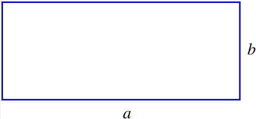
Määritelmä: Suunnikkaan pinta-ala
Suunnikkaan pinta-ala on
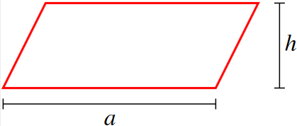
Määritelmä: Kolmion pinta-ala
Kolmion pinta-ala on (määritelmän mukaan) \[ A=\frac{1}{2}ah. \]
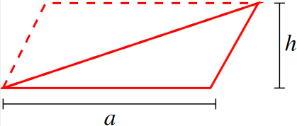
Monikulmio
(Yksinkertainen) monikulmio on tasojoukko, jota rajaa äärellisestä määrästä peräkkäisiä janoja koostuva suljettu käyrä. Vain peräkkäiset janat saavat leikata toisiaan yhteisessä päätepisteessä.
Määritelmä: Monikulmion pinta-ala
Monikulmion pinta-ala määritellään jakamalla se
äärelliseen määrään kolmioita (monikulmion
Lause.
Kolmioiden pinta-alojen summaf ei riipu monikulmion kolmioinnin valinnasta.
Yleinen tapaus
Tasojoukolle \(\color{red} D\), jota rajaa umpinainen itseään leikkaamaton käyrä, voidaan muodostaa sisämonikulmioita \(\color{blue}P_i\) ja ulkomonikulmioita \(P_o\): \(\color{blue}P_i\color{black} \subset \color{red}D\color{black}\subset P_o\).
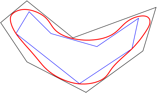
Yllätys: Se, että joukkoa \(D\) rajoittaa umpinainen (itseään leikkaamaton) käyrä, ei takaa, että joukon pinta-ala on määritelty: Reunakäyrä voi olla niin "mutkitteleva", että sillä on positiivinen "pinta-ala". Ensimmäisen esimerkin konstruoi [W.F. Osgood, 1903]:
Wikipedia: Osgood curveEsimerkki
Johda \(R\)-säteisen ympyrän pinta-alan kaava \(A=\pi R^2\) valitsemalla sisä- ja ulkomonikulmioiksi säännöllisiä \(n\)-kulmioita, ja ottamalla lopuksi raja-arvo \(n\to\infty\).
Ratkaisu: vapaaehtoinen lisätehtävä, jossa tarvitaan raja-arvoa \[\lim_{x\to 0}\frac{\sin x}{x} = 1.\] Vihje: Osoita, että säännöllisten sisä- ja ulkomonikulmioiden pinta-alat ovat \[ \pi R^2\frac{\sin (2\pi/n)}{2\pi/n} \ \text{ ja }\ \pi R^2\frac{\tan \pi/n}{\pi/n}.\]
8. Integral
From sum to integral
Definite integral
Geometric interpretation: Let \(f\colon[a,b]\to\mathbb{R}\) be such that \(f(x)\ge 0\) for all \(x\in[a,b]\). How can we find the area of the region bounded by the function graph \(y=f(x)\), the x-axis and the two lines \(x=a\) and \(x=b\)?
The answer to this question is given by the definite integral \[\int_{a}^{b}f(x)\,dx\] Remark. The general definition of the integral does not necessitate the condition \(f(x)\ge 0\).
Integration of continuous functions
Definition: Partition
Let \(f\colon[a,b]\to\mathbb{R}\) be continuous. A finite sequence \(D=(x_{0},x_{1},x_{2},\dots,x_{n})\) of real numbers such that \[a=x_{0} < x_{1} < x_{2} < \dots < x_{n} = b\] is called a partition of the interval \([a,b]\).
Definition: Upper and lower sum
For each partition \(D\) we define the related upper sum of the function \(f\) as \[U_{D}(f) = \sum_{k=1}^{n}M_{k}(x_{k}-x_{k-1}),~M_{k} = \max\{f(x)\mid x_{k-1}\le x\le x_{k}\}\] and the lower sum as \[L_{D}(f) = \sum_{k=1}^{n}m_{k}(x_{k}-x_{k-1}),~m_{k}=\min\{f(x)\mid x_{k-1}\le x\le x_{k}\}.\]
If \(f\) is a positive function then the upper sum represents the total area of the rectangles circumscribing the function graph and similarly the lower sum is the total area of the inscribed rectangles.
Properties of partitions
- Suppose that \(D_{1}\) and \(D_{2}\) are two partitions of a given interval such that \(D_{1}\) is a subsequence of
\(D_{2}\) (i.e. \(D_{2}\) is finer than \(D_{1}\)). Then the inequalities
\(U_{D_1}(f) \ge U_{D_{2}}(f)~\) and \(~L_{D_{1}}(f) \le L_{D_{2}}(f)\)
always hold. - For any two partitions \(D_{1}\) and \(D_{2}\) of a given interval the inequality \[ L_{D_{2}}(f) \le U_{D_{1}}(f)\] always holds.
\(f(x)=~\)
| Upper Darboux sum | Lower Darboux sum |
Definition: Integrability
We say that a function \(f\colon[a,b]\to\mathbb{R}\) is integrable if for every \(\epsilon>0\) there exists a corresponding partition \(D\) of \([a,b]\) such that \[ U_{D}(f) - L_{D}(f) < \epsilon.\]
Definition: Integral
Integrability implies that there exists a unique real number \(I\) such that \(L_{D}(f)\le I\le U_{D}(f)\) for every partition \(D\). This is called the integral of \(f\) over the interval \([a,b]\) and denoted by \[ I = \int_{a}^{b}f(x)\,dx. \]
Remark. This definition of the integral is sometimes referred to as the Darboux integral.
For non-negative functions \(f\) this definition of the integral coincides with the idea of making the difference between the the areas of the circumscribed and the inscribed rectangles arbitrarily small by using ever finer partitions.
Theorem.
A continuous function on a closed interval is integrable.
Here we will only provide the proof for continuous functions with bounded derivatives.
Suppose that \(f\colon[a,b]\to\mathbb{R}\) is a continuous function and that there exists a constant \(L>0\) such that \(|f'(x)|\le L\) for all \(x\in]a,b[\). Let \(\epsilon>0\) and define \(D\) to be an equally spaced partition of \([a,b]\) such that \[\underbrace{|x_{k}-x_{k-1}|}_{=\Delta x} < \frac{\epsilon}{L(b-a)},~\text{for all} k=1,2,\dots,n.\] Let \(f(y_{k})=m_{k}\) and \(f(z_{k})=M_{k}\) for some suitable points \(y_{k},z_{k}\in[x_{k-1},x_{k}]\). The mean value theorem then states that \[M_{k}-m_{k}=f'(c_{k})|z_{k}-y_{k}|\le L\Delta x<\frac{\epsilon}{b-a}.\] and thus \[U_{D}(f)-L_{D}(f) = \sum_{k=1}^{n}(M_{k}-m_{k})\Delta x < \frac{\epsilon}{b-a}\sum_{k=1}^{n}\Delta x = \epsilon.\]
\(\square\)
Definition: Riemann integral
Suppose that \(f\colon[a,b]\to\mathbb{R}\) is a continuous function and let \((x_{0},x_{1},\dots,x_{n})\) be a partition of \(\left[a,b\right]\) and \((z_{1},z_{2},\dots,z_{n})\) be a sequence of real numbers such that \(z_{k}\in[x_{k-1},x_{k}]\) for all \(1\le k\le n\). The partial sums \[ S_{n} = \sum_{k=1}^{n}f(z_{k})\Delta x_{k},~\text{where} ~\Delta x_{k}=x_{k}-x_{k-1} \] are called the Riemann sums of \(f\). Suppose further that the partitions are such that \(\displaystyle\max_{1\le k\le n}\Delta x_{k}\to 0\) as \(n\to\infty\). The integral of \(f\) can then be defined as the limit \[ \int_{a}^{b}f(x)\,\mathrm{d}x = \lim_{n\to\infty} S_{n}. \] This definition of the integral is called the Riemann integral.
Remark. This definition of the integral turns out to be equivalent to that of the Darboux integral i.e. a function is Riemann-integrable if and only if it is Darboux-integrable and the values of the two integrals are always equal.
Example
Find the integral of \(f(x)=x\) over the interval \([0,1]\) using Riemann sums.
Let \(x_{k}=k/n\). Then \(x_{0}=0\), \(x_{n}=1\) and \(x_{k} < x_{k+1}\) for all \(0\le k\le n\). Thus the sequence \((x_{0},x_{1},x_{2},\dots,x_{n})\) is a proper partition of \(\left[0,1\right]\). This partition has the pleasant property hat \(\Delta x=1/n\) is a constant. Estimating the Riemann sums we now find that \[\sum_{k=1}^{n}f(x_{k})\Delta x = \sum_{k=1}^{n}x_{k}\Delta x= \sum_{k=1}^{n}\frac{k}{n}\left(\frac{1}{n}\right)\] \[= \frac{1}{n^2}\sum_{k=1}^{n}k = \frac{1}{n^2}\frac{n(n+1)}{2} = \frac{n+1}{2n}\to \frac{1}{2},\] as \(n\to\infty\) and hence \[\int_{0}^{1}f(x)\,\mathrm{d}x = \frac{1}{2}.\]
This is of course the area of the triangular region bounded by the line \(y=x\), the \(x\)-axis and the lines \(x=0\) and \(x=1\).
Remark. Any interval \([a,b]\) can be partitioned into equally spaced subintervals by setting \(\Delta x = (b-a)/n\) and \(x_{k} = a + k\Delta x\).
Conventions
- If the upper and lower limits of integration are the same then the integral is zero: \[ \int_{a}^{a}f(x)\,dx = 0.\]
- Reversing the limits of integration changes the sign of the integral: \[ \int_{b}^{a}f(x)\,dx = -\int_{a}^{b}f(x)\,dx.\]
- It also follows that \[ \int_{a}^{b}f(x)\,dx = \int_{a}^{c}f(x)\,dx + \int_{c}^{b}f(x)\,dx \] holds for all \(a,b,c\in\mathbb{R}\).
Piecewise-defined functions
Definition: Piecewise continuity
A function \(f\colon\left[a,b\right]\to\mathbb{R}\) is called piecewise continuous if it is continuous except at a finite number of points \[a\le c_{1} < c_{2} < \dots < c_{m} \le b\] and the one-sided limits of the function are defined and bounded on each of these points. It follows that the restriction of \(f\) on each subinterval \(\left[c_{k-1},c_{k}\right]\) is continuous if the one-sided limits are taken to be the values of the function at the end points of the subinterval.
Definition: Piecewise integration
Let \(f\colon\left[a,b\right]\) be a piecewise continuous function. Then \[\int_{a}^{b}f(x)\,dx = \sum_{k=1}^{m+1}\int_{c_{k-1}}^{c_{k}}f(x)\,dx,\] where \(a=c_{0}< c_{1} < \dots < c_{m+1} = b\) and \(f\) is thought as a continuous function on each subinterval \(\left[c_{k-1},c_{k}\right]\). Usually functions which are continuous yet piecewise defined are also integrated using the same idea.
Example
Consider the function \(f\colon\left[-1,1\right]\) defined as \[ f(x) = \begin{cases} -1 &\text{ for }-1\le x<0 \\ 1 &\text{ for }0\le x\le 1. \end{cases} \] We can now integrate \(f\) as follows: \[ \int_{-1}^{1}f(x)\,dx = \int_{-1}^{0}f(x)\,dx + \int_{0}^{1}f(x)\,dx \] \[ =\int_{-1}^{0}(-1)\,dx + \int_{0}^{1}1\,dx = -1\cdot(-1-0) + 1\cdot(1-0) = 2. \]
Important properties
Properties
Suppose that \(f,g\colon\left[a,b\right]\to\mathbb{R}\) are piecewise continuous functions. The integral has the following properties
- Linearity: If \(c_{1},c_{2}\in\mathbb{R}\) then \[\int_{a}^{b}\big(c_{1}f(x)+c_{2}g(x)\big)\,\mathrm{d}x = c_{1}\int_{a}^{b}f(x)\,\mathrm{d}x+c_{2}\int_{a}^{b}g(x)\,\mathrm{d}x.\]
- If \(h(x)\ge 0\) for all \(x\in[a,b]\) then \[\int_{a}^{b}h(x)\,\mathrm{d}x \ge 0.\]
- If \(f(x)\le g(x)\) then \[\int_{a}^{b}f(x)\,\mathrm{d}x \le \int_{a}^{b}g(x)\,\mathrm{d}x.\]
- As \(f(x)\le|f(x)|\) it follows that \[\int_{a}^{b}f(x)\,\mathrm{d}x \le \int_{a}^{b}|f(x)|\,\mathrm{d}x\] and taking the absolute value of both sides of the equation gives \[\left|\int_{a}^{b}f(x)\,\mathrm{d}x\right|\le \int_{a}^{b}|f(x)|\,\mathrm{d}x.\]
- Suppose that \(p=\inf_{x\in\left[a,b\right]}f(x)\) and \(s=\sup_{x\in\left[a,b\right]}f(x)\). Then \[p(b-a)\le \int_{a}^{b}f(x)\,dx \le s(b-a).\]
Fundamental theorem of calculus
Theorem: Mean value theorem
Let \(f\colon[a,b]\to\mathbb{R}\) be a continuous function. Then there exists \(c\in(a,b)\) such that \[ f(c)=\frac{1}{b-a}\int_{a}^{b}f(x)\,\mathrm{d}x.\] This is the mean value of \(f\) on the interval \([a,b]\) and we denote it with \(\overline{f}\).
Suppose that \(m\) and \(M\) are the minimum and maximum of \(f\) on the interval \([a,b]\), respectively. It follows that \[ m(b-a)\le \int_{a}^{b}f(x)\,\mathrm{d}x\le M(b-a)\] or \[m\le \frac{1}{b-a}\int_{a}^{b}f(x)\,\mathrm{d}x\le M\quad \Leftrightarrow\quad m\le \overline{f}\le M.\] Thus \(\overline{f}\) is between the minimum and maximum of a continuous function \(f\) and by the intermediate value theorem it must be that \(f(c)=\overline{f}\) for some \(c\in\,]a,b[\).
\(\square\)
(First) Fundamental theorem of calculus.
Let \(f\colon[a,b]\to\mathbb{R}\) be a continuous function. Then \[ \frac{\mathrm{d}}{\mathrm{d}x}\int_{a}^{x}f(t)\,\mathrm{d}t = f(x)\] for all \(x\in\,]a,b[\).
Let \[ F(x) = \int_{a}^{x}f(t)\,\mathrm{d}t. \] The mean value theorem implies that there exists \(c\in\,[x,x+h]\) such that \[ \frac{F(x+h)-F(x)}{h} = \frac{1}{h}\left(\int_{a}^{x+h}f(t)\, \mathrm{d}t-\int_{a}^{x}f(t)\,\mathrm{d}t\right)\] \[ =\frac{1}{h}\int_{x}^{x+h}f(t)\,\mathrm{d}t = \frac{1}{h}f(c)(x+h-x) = f(c). \] As \(h\to0\) we see that \(c\to x\) and from the continuity of \(f\) it follows that \(f(c)\to f(x)\). Thus \(F'(x)=f(x)\).
\(\square\)
Antiderivative
If \(F'(x)=f(x)\) on some open interval then \(F\) is the antiderivative (or the primitive function) of \(f\). The fundamental theorem of calculus guarantees that for every continuous function \(f\) there exists an antiderivative \[ F(x) = \int_{a}^{x}f(t)\,dt. \] The antiderivative is not necessarily expressible as a combination of elementary functions even if \(f\) were an elementary function, e.g. \(f(x) = e^{-x^{2}}\). Such primitives are called nonelementary antiderivatives.
Theorem.
Antiderivatives are only unique up to a constant; \[\int f(x)\,dx = F(x) + C, C\in\mathbb{R} \text{ constant }\] if \(F'(x)=f(x)\).
Suppose that \(F'_{1}(x)=F'_{2}(x)=f(x)\) for all \(x\). Then the derivative of \(F_{1}(x)-F_{2}(x)\) is identically zero and thus the difference is a constant.
\(\square\)
(Second) Fundamental theorem of calculus
Let \(f\colon\left[a,b\right]\to\mathbb{R}\) be a continuous function and \(G\) an antiderivative of \(f\), then \[\int_{a}^{b}f(x)\,dx = G(x)\Big|_{x=a}^{x=b} = G(b)-G(a). \]
Because \(F(x)=\int_{a}^{x}f(t)\,dt\) is an antiderivative of \(f\) then due to continuity \(F(x)-G(x)=C=\text{constant}\) for all \(x\in\left[a,b\right]\). Substituting \(x=a\) we find that \(C=-G(x)\). Thus \[\int_{a}^{x}f(t)\,dt = F(x) = G(x)-G(a)\] and substituting \(x=b\) the result follows.
\(\square\)
Suppose that \(f\) is a continuous function and that \(a\) and \(b\) are differentiable functions. Then \[\frac{d}{dx}\int_{a(x)}^{b(x)}f(t)\,dt = f(b(x))b'(x)-f(a(x))a'(x).\]
Suppose that \(F\) is an antiderivative of \(f\). Then from the fundamental theorem of calculus and the chain rule it follows that \[\frac{d}{dx}\int_{a(x)}^{b(x)}f(t)\,dt = \frac{d}{dx}\big(F(b(x)) - F(a(x))\big)\] \[=\frac{d}{dx}F(b(x)) - \frac{d}{dx}F(a(x)) = F'(b(x))b'(x) - F'(a(x))a'(x) \] \[ = f(b(x))b'(x) - f(a(x))a'(x). \]
\(\square\)
Integrals of elementary functions
Constant Functions
Given the constant function \(f(x) = c,\,c\in\mathbb{R}\). The integral \(\int\limits_a^b f(x)\,\mathrm{d} x = \int\limits_a^b c \, \mathrm{d}x\) has to be determined now.
Solution by finding a antiderivative
From the previous chapter it is known that \(g(x) = c\cdot x\) gives \(g'(x) = c\). This means that \(c \cdot x\) is an antiderivative for \(c\). So the following applies \[\int\limits_a^b c \, \mathrm{d}x = [c \cdot x]_{x=a}^{x=b} = c\cdot b - c \cdot a = c \cdot (b-a).\]
Remark: Of course, a function \(h(x) = c \cdot x + d\) would also be an antiderivative of \(f\), since the constant \(d\) is omitted in the derivation. For sake of simplicity \(c \cdot x\) can be used, since \(d\) can be chosen as \(d=0\) for definite integrals.
Solution by geometry
The area under the constant function forms a rectangle with height \(c\) and length \(b-a\). Thus the area is \(c \cdot (b-a)\) and this corresponds to the solution of the integral. Illustrate this remark by a sketch.
Linear functions
Given is the linear function \( f(x) = mx\). We are looking for the integral \(\int\limits_a^b f(x)\, \mathrm dx=\int\limits_a^b mx\, \mathrm dx\).
Solve by finding a antiderivative
The antiderivative of a linear function is in any case a quadratic function, since \(\frac{\mathrm d x^2}{\mathrm dx} = 2x \). The derivative of a quadratic function results in a linear function. Here, it is important to consider the leading factor as in \[\frac{\mathrm d (m \cdot \frac{1}{2} \cdot x^2)}{\mathrm dx} = mx.\] Thus the result is \[\int\limits_a^b mx \mathrm{d}x = \left[\frac{m}{2}x^2 \right]_{x=a}^{x=b}= \frac{m}{2}b^2 - \frac{m}{2}a^2. \]
Solving by geometry
The integral \(\int\limits_a^b mx\, \mathrm dx\) can be seen geometrically, as subtracting the triangle with the edges \((0|0)\), \((a|0)\) and \((a| ma)\) from the triangle with the edges \((0|0)\), \((b|0)\) and \((b| mb)\). Since the area of a triangle ist given by \(\frac{1}{2} \cdot \mbox{baseline} \cdot \mbox{height}\), the area of the first triangle \(\frac{1}{2}\cdot b \cdot mb = \frac{1}{2}mb^2\) and that of the second triangle is analogous \(\frac{1}{2}ma^2\). For the integral the result is \(\frac{m}{2}b^2 - \frac{m}{2}a^2\). This is consistent with the integral calculated using the antiderivative. Illustrate this remark by a sketch.
Power functions
In constant and linear functions we have already seen that the exponent of a function decreases by one when it is derived. So it has to get bigger when integrating. The following applies: \[\frac{\mathrm d x^n}{\mathrm dx} = n \cdot x^{n-1}. \] It follows that the antiderivative for \(x^n\) must have the exponent \(n+1\), \[\frac{\mathrm d x^{n+1}}{\mathrm dx} = (n+1) \cdot x^n.\] By multiplying the last equation with \(\frac{1}{n+1}\) we get \[\frac{\mathrm d}{\mathrm dx}\frac{1}{n+1} x^{n+1} = \frac{n+1}{n+1} \cdot x^n = x^n.\] Finally the antiderivative is \(\int x^n\, \mathrm dx = \frac{1}{n+1} x ^{n+1}+c,\,c\in\mathbb{R}\).
Examples
- \(\int x^2\, \mathrm dx = \frac{1}{3} x^3 +c,\,c\in\mathbb{R}\)
- \(\int x^3\, \mathrm dx = \frac{1}{4} x^4 +c,\,c\in\mathbb{R}\)
- \(\int x^{20}\, \mathrm dx = \frac{1}{21} x^{21} +c,\,c\in\mathbb{R}\)
The formula \(\int x^n\, \mathrm dx = [\frac{1}{n+1} x^{n+1}] \) is also valid, if the exponent of the function is a real number and not equal \(-1\).
Examples
- \(\int x^{2,7}\, \mathrm dx = \frac{1}{3,7} x^{3,7}+c,\,c\in\mathbb{R}\)
- \(\int \sqrt{x}\, \mathrm dx = \int x^\frac{1}{2} = \frac{2}{3} x^{\frac{3}{2}}+c,\,c\in\mathbb{R}\)
- But: For \(x\gt0\) applies\(\int x^{-1}\,\mathrm d x=\ln(x)+c,\,c\in\mathbb{R}.\)
Natural Exponential function
The natural exponential function \(f(x) = e^x\) is one of the easiest function to differentiate and integrate. Since the derivation of \(e^x\) results in \(e^x\), it follows \[\int e^x\, \mathrm dx = e^x +c, \, c\in \mathbb{R}.\]
Example 1
Determine the value of the integral \(\int_0^1 e^z \,\mathrm{d} z\).
\[\int\limits_0^1e^z\,\mathrm{d}z= e^z\big|_{z=0}^{z=1}=e^1-e^0=e-1.\]
Example 2
Determine the value of the integral \(\int_0^b e^{\alpha t} \,\mathrm{d} t\). Using the same considerations as above we get \[\int\limits_0^b e^{\alpha t}\,\mathrm{d}t= \frac{1}{\alpha}e^{\alpha t}\big|_{t=0}^{t=b} =\frac{1}{\alpha}\left(e^{\alpha b}-e^0\right)=\frac{1}{\alpha}\left(e^{\alpha b}-1\right).\] Important is here, that we have to use the factor \(\frac1{\alpha}\).
Natural Logarithm
The derivative of the natural logarithmic function is \(\ln'(x) =\frac{1}{x}\) for \(x\gt0\). It even applies \(\ln'(x) =\frac{1}{x}\) to \(x<0\). These results together result in for the antiderivative of \(\frac{1}{x}\)
\[\int \frac{1}{x}\,\mathrm{d}x = \ln\left(|x|\right) +c , c\in\mathbb{R}.\]
An antiderivative can be specified for the natural logarithm: \[\int \ln(x)\,\mathrm{d}x = x\ln(x) - x + c ,\, c\in\mathbb{R}.\]
Trigonometric function
The antiderivatives of \(\sin(x)\) and \(\cos(x)\) also result logically if you derive "backwards". We have \[\int \sin(x)\, \mathrm dx = -\cos(x)+c,\,c\in\mathbb{R},\] since \( (-\cos(x))' =-(-\sin(x))=\sin(x).\) Furthermore we know \[\int \cos(x)\, \mathrm dx = \sin(x)+c,\,c\in\mathbb{R},\] since \((\sin(x))' = \cos(x) \) applies.
Example 1
Which area is covered by the sine on the interval \([0,\pi]\) and the \(x\)-axis? To determination the area we simply have to evaluate the integral \[\int_0^{\pi} \sin(\tau) \, \mathrm{\tau}.\] That means \[\int_0^{\pi} \sin(\tau) \, \mathrm{d}\tau = \left[-\cos(\tau)\right]_{\tau=0}^{\tau=\pi} = -\cos(\pi) - (-\cos(0)) = -(-1) - (-1) = 2.\] Again make a sketch for this example.
Example 2
How can the integral \(\int \cos(\omega t +\phi)\,\mathrm{d}t\) be expressed analytically?
To determine the integral we use the antiderivative of the cosine: \(\sin'(x) = \cos(x)\). However, the inner derivativ has to be considered in the given function and thus we get \[\int \ \cos(\omega t +\phi)\,\mathrm{d}t =\frac{1}{\omega}\sin(\omega t+\phi)+c,\,c\in\mathbb{R}.\]
Summary:
The most common antiderivatives follow from the rules of differentiation: \[\int x^{r}\,dx = \frac{1}{r+1}x^{r+1} + C, ~r\neq-1\] \[\int x^{-1}\,dx = \ln|x| + C\] \[\int e^{x}\,dx = e^{x} + C\] \[\int \sin x\,dx = -\cos x + C\] \[\int \cos x\,dx = \sin x + C\] \[\int \frac{dx}{1+x^{2}} = \arctan x + C\]
Example 1
Evaluate the integrals \(\displaystyle \int_{-1}^{1}e^{-x}\,dx\) and \(\displaystyle\int_{0}^{1}\sin(\pi x)\,dx\).
Solution. The antiderivative of \(e^{-x}\) is \(-e^{-x}\) so we have that \[\int_{-1}^{1}e^{-x}\,dx = -e^{-1}+e^{1} = 2\sinh1.\] The antiderivative of \(\sin(\pi x)\) is \(-\frac{1}{\pi}\cos(\pi x)\) and thus \[\int_{0}^{1}\sin(\pi x)\,dx = -\frac{1}{\pi}(\cos\pi-\cos0) = \frac{2}{\pi}.\]
Example 2
Evaluate the integral \(\displaystyle\int_{0}^{1}\frac{x}{\sqrt{25-9x^{2}}}\,dx\).
Solution. The antiderivative might look something like \(F(x)=a(25-9x^{2})^{1/2}\), where we can find the factor \(a\) through differentiation: \[D\big(a(25-9^{2})^{1/2}\big) = a\cdot\frac{1}{2}\cdot(-18x)(25-9x^{2})^{-1/2} = \frac{-9ax}{\sqrt{25-9x^{2}}}\] hence if \(a=-1/9\) we get the correct antiderivative. Thus \[\int_{0}^{1}\frac{x}{\sqrt{25-9x^{2}}}\,dx = -\frac{1}{9}\cdot(25-9x^{2})^{1/2}\Big|_{x=0}^{x=1} = -\frac{1}{9}(\sqrt{16}-\sqrt{25}) = \frac{1}{9}.\] This integral can also be solved using integration by substitution; more on this method later.
Geometric applications
Area of a plane region
Suppose that \(f\) and \(g\) are piecewise continuous functions. The area of a region bounded by the graphs \(y=f(x)\), \(y=g(x)\) and the vertical lines \(x=a\) and \(x=b\) is given by the integral \[A=\int_{a}^{b}|f(x)-g(x)|\,dx.\]
Especially if \(f\) is a non-negative function on the interval \([a,b]\) and \(g(x)=0\) for all \(x\) then the integral \[A=\int_{a}^{b}f(x)\,dx\] is the area of the region bounded by the graph \(y=f(x)\), the \(x\)-axis and the vertical lines \(x=a\) and \(x=b\).
Arc length
The arc length \(\ell\) of a planar curve \(y=f(x)\) between points \(x=a\) and \(x=b\) is given by the integral \[\ell = \int_{a}^{b}\sqrt{1+f'(x)^{2}}\,dx.\]
Heuristic reasoning: On a small interval \(\left[x,x+\Delta x\right]\) the arc length of the curve between \(y=f(x)\) and \(y=f(x+\Delta x)\) is approximately \[\Delta s \approx \sqrt{\Delta x^{2} + \Delta y^{2}} = \Delta x\sqrt{1+\left(\frac{\Delta y}{\Delta x}\right)^{2}} \approx \Delta x\sqrt{1+f'(x)^{2}}.\]
Surface of revolution
The area of a surface generated by rotating the graph \(y=f(x)\) around the \(x\)-axis on the interval \(\left[a,b\right]\) is given by \[A = 2\pi\int_{a}^{b}|f(x)|\sqrt{1+f'(x)^{2}}\,dx.\] Heuristic reasoning: An area element of the surface is approximately \[\Delta A \approx \text{perimeter}\cdot\text{length} = 2\pi|f(x)|\cdot\Delta s.\]
Solid of revolution
Suppose that the cross-sectional area of a solid is given by the function \(A(x)\) when \(x\in\left[a,b\right]\). Then the volume of the solid is given by the integral \[V = \int_{a}^{b}A(x)\,dx.\] If the graph \(y=f(x)\) is rotated around the \(x\)-axis between the lines \(x=a\) and \(x=b\) the volume of the generated figure (the solid of revolution) is \[V = \pi\int_{a}^{b}f(x)^{2}\,dx.\] This follows from the fact that the cross-sectional area of the figure at \(x\) is a circle with radius \(f(x)\) i.e. \(A(x)=\pi f(x)^{2}\).
More generally: Let \(0\le g(x)\le f(x)\) and suppose that the region bounded by \(y=f(x)\) and \(y=g(x)\) and the lines \(x=a\) and \(x=b\) is rotated around the \(x\)-axis. The volume of this solid of revolution is \[V = \pi\int_{a}^{b}\big(f(x)^{2}-g(x)^{2}\big)\,dx.\]
Improper integral
Definition: Improper integral
- 1st kind: The integral is defined on an unbounded domain, \(\left[a,\infty\right[,\left]-\infty,b\right]\) or the entire \(\mathbb{R}\).
- 2nd kind: The integrand function is unbounded in the domain of integration or a two-sided limit doesn't exist on one or both of the endpoints of the integral
One limitation of the improper integration is that the limit must be taken with respect to one endpoint at a time.
Example
\[\int_{0}^{\infty}\frac{dx}{\sqrt{x}(1+x)} = \int_{0}^{1}\frac{dx}{\sqrt{x}(1+x)} + \int_{1}^{\infty}\frac{dx}{\sqrt{x}(1+x)}\] Provided that both of the integrals on the right-hand side converge. If either of the two is divergent then so is the integral.
Definition
Let \(f\colon\left[a,\infty\right[\to\mathbb{R}\) be a piecewise continuous function. Then \[\int_{a}^{\infty}f(x)\,dx = \lim_{R\to\infty}\int_{a}^{R}f(x)\,dx\] provided that the limit exists and is finite. We say that the improper integral of \(f\) converges over \(\left[a,\infty\right[\).
Likewise for \(f\colon\left]-\infty,b\right]\to\mathbb{R}\) we define \[\int_{-\infty}^{b}f(x)\,dx = \lim_{R\to\infty}\int_{-R}^{b}f(x)\,dx\] provided that the limit exists and is finite.
Example
Find the value of \(\displaystyle\int_{0}^{\infty}e^{-x}\,dx\).
Solution. Notice that \[\int_{0}^{R}e^{-x}\,dx = \left(-e^{-x}\right)\Bigg|_{x=0}^{R}=1-e^{-R}\to 1\] as \(R\to\infty\). Thus the improper integral converges and \[\int_{0}^{\infty}e^{-x}\,dx = 1.\]
Definition
Let \(f\colon\mathbb{R}\to\mathbb{R}\) be a piecewise continuous function. Then \[\int_{-\infty}^{\infty}f(x)\,dx = \int_{-\infty}^{0}f(x)\,dx + \int_{0}^{\infty}f(x)\,dx\] if both of the two integrals on the right-hand side converge.
In the case \(f(x)\ge0\) for all \(x\in\mathbb{R}\) the following holds \[\int_{-\infty}^{\infty}f(x)\,dx = \lim_{R\to\infty}\int_{-R}^{R}f(x)\,dx.\]
However, this doesn't apply in general. For example, let \(f(x)=x\). Note that even though \[ \int_{-R}^{R}f(x)\,dx = \int_{-R}^{R}x\,dx = \frac{R^2}{2} - \frac{(-R)^2}{2} = 0 \] for all \(R\in\mathbb{R}\) the improper integral \[ \int_{-\infty}^{\infty}x\,dx = \lim_{R\to\infty}\int_{-R}^{0}x\,dx + \lim_{R\to\infty}\int_{0}^{R}x\,dx = \lim_{R\to\infty}-\frac{(-R)^2}{2} + \lim_{R\to\infty}\frac{R^2}{2} = \infty - \infty \] does not converge.
Improper integrals of the 2nd kind are handled in a similar way using limits. As there are many different (but essentially rather similar) cases, we leave the matter to one example only.
Example
Find the value of the improper integral \(\displaystyle\int_{0}^{1}\frac{dx}{\sqrt{x}}\).
Solution. We get \[\int_{\epsilon}^{1}\frac{dx}{\sqrt{x}} = \left(2\sqrt{x}\right)\Bigg|_{x=\epsilon}^{x=1} = 2-2\sqrt{\epsilon} \to 2,\] as \(\epsilon\to0+\). Thus the integral converges and its value is \(2\).
Comparison test
Theorem.
Suppose that \(f\) and \(g\) are integrable functions such that \(|f(x)|\le g(x)\) for \(a < x < b\).- If the improper integral \[I=\int_{a}^{b}g(x)\,dx\] converges then so does \(\displaystyle\int_{a}^{b}f(x)\,dx\) and its value is less than or equal to \(I\).
- If the improper integral \[\int_{a}^{b}f(x)\,dx\] diverges then so does \(\displaystyle\int_{a}^{b}g(x)\,dx\).
Example 2
Notice that \[0\le\frac{1}{\sqrt{x}(1+x)}\le\frac{1}{\sqrt{x}}, \text{ for }0 < x < 1\] and that the integral \[\int_{0}^{1}\frac{dx}{\sqrt{x}} = 2\] converges. Thus by the comparison test the integral \[\int_{0}^{1}\frac{dx}{\sqrt{x}(1+x)}\] also converges and its value is less than or equal to \(2\).
Example 3
Likewise \[0\le\frac{1}{\sqrt{x}(1+x)} < \frac{1}{\sqrt{x}(0+x)}=\frac{1}{x^{3/2}}, \text{ for }x\ge1\] and because \(\displaystyle\int_{1}^{\infty}x^{3/2}\,dx=2\) converges so does \[\int_{1}^{\infty}\frac{dx}{\sqrt{x}(1+x)}\] and its value is less than or equal to \(2\).
Note. The choice of the dominating function depends on both the original function and the interval of integration.
Example 4
Determine whether the integral \[\int_{0}^{\infty}\frac{x^2+1}{x^3(\cos^2{x}+1)}\,dx\] converges or diverges.
Solution. Notice that \(x^2+1\ge x^2\) for all \(x\in\mathbb{R}\) and therefore \[\frac{x^2+1}{x^3(\cos^2{x}+1)} \ge \frac{1}{x\underbrace{(\cos^2{x}+1)}_{\le 2}} \ge \frac{1}{2x}.\] Now, because the integral \(\displaystyle\int_{0}^{\infty}\frac{dx}{2x}\) diverges then by the comparison test so does the original integral.
Integration techniques
Logarithmic integration
Given a quotient of differentiable functions, we know to apply the quotient rule. However, this is not so easy with integration. Here only for a few special cases we will state rules in this chapter.
Logarithmic integration As we already know the derivative of \(\ln(x)\), i.e. the natural logarithm to the base \(e\), equal to \(\frac{1}{x}\). According to the chain rule the derivative of differentiable function with positive function values is \(f\,:\,\frac{\mathrm d}{\mathrm dx} \ln (f(x)) = \frac{f'(x)}{f(x)}\). This means that for a quotient of functions where the numerator is the derivative of the denominator yields the rule: \begin{equation} \int \frac{f'(x)}{f(x)}\, \mathrm{d} x= \ln \left(|f(x)|\right) +c,\,c\in\mathbb{R}.\end{equation} Using the absolute value of the function is important, since the logarithm is defined on \(\mathbb{R}^+\).
Examples
- \(\int \frac{1}{x}\, \mathrm dx = \int \frac{x'}{x} \mathrm\, dx = \ln(|x|) +c,\,c\in\mathbb{R} \).
- \(\int \frac{3x^2 + 17}{x^3 +17x - 15}\, \mathrm dx = \ln(|x^3 + 17x - 15|)+c,\,c\in\mathbb{R}\).
- \(\int \frac{\cos(x)}{\sin(x)}\,\mathrm dx = \ln(|\sin(x)|)+c,\,c\in\mathbb{R}\).
Integration of rational functions - partial fraction decomposition
The logarithmic integration works well in special cases of broken rational functions where the counter is a multiple of the derivation of the denominator. However, other cases can sometimes be traced back to this. This method is called partial fractional decomposition, which represents rational functions as the sum of proper rational functions.
Example 1
The function \(\frac{1}{1-x^2}\) cannot be integrated at first glance. However, the denominator \(1-x^2\) can be written as \((1-x)(1+x)\) and the function can finally reads as \(\dfrac{1}{1-x^2} = \dfrac{\frac{1}{2}}{1+x} + \dfrac{\frac{1}{2}}{1-x}\) by partial fraction decomposition. This expression can be integrated, as demonstrated now: \begin{eqnarray} \int \dfrac{1}{1-x^2} \,\mathrm dx &= & \int \dfrac{\frac{1}{2}}{1+x} + \dfrac{\frac{1}{2}}{1-x}\, \mathrm dx \\ & =& \frac{1}{2} \int \dfrac{1}{1+x}\, \mathrm dx - \frac{1}{2} \int \dfrac{-1}{1-x}\, \mathrm dx\\ & = &\frac{1}{2} \ln|1+x| +c_1 - \frac{1}{2} \ln|1-x| +c_2\\ &= &\frac{1}{2} \ln \left|\dfrac{1+x}{1-x}\right|+c,\,c\in\mathbb{R}. \end{eqnarray} This procedure is now described in more detail for some special cases.
Case 1: \(Q(x)=(x-\lambda_1)(x-\lambda_2)\) with \(\lambda_1\ne\lambda_2\). In this case, \(R\) has the representation \(R(x) = \frac{ax+b}{(x-\lambda_1)(x-\lambda_2)}\) and can be transformed to \[\frac{ax+b}{(x-\lambda_1)(x-\lambda_2)} = \frac{A}{(x-\lambda_1)}+\frac{B}{(x-\lambda_2)}.\] By multiplying with \((x-\lambda_1)(x-\lambda_2)\) it yields ot \[ax+b = A(x-\lambda_1) + B(x-\lambda_2) = \underbrace{(A+B)}_{\stackrel{!}{=}a}x + \underbrace{(-A\lambda_1-B\lambda_2)}_{\stackrel{!}{=}b}.\]
\(A\) and \(B\) are now obtained by the method of equating the coefficients.
Example 2
Determe the partial fraction decomposition of \(\frac{2x+3}{(x-4)(x+5)}\).
Start with the equation \[\frac{2x+3}{(x-4)(x+5)} = \frac{A}{(x-4)}+\frac{B}{(x+5)}\] to get the parameters \(A\) and \(B\). Multiplication by \({(x-4)(x+5)}\) leads to \[2x+3 = A(x+5)+B(x-4) = (A+B)x +5A -4B.\] Now we get the system of linear equations
\begin{eqnarray}A+B & = & 2 \\ 5A - 4 B &=& 3\end{eqnarray} with the solution \(A = \frac{11}{9}\) and \(B= \frac{7}{9}\). The representation with proper rational functions is \[\frac{2x+3}{(x-4)(x+5)}=\frac{11}{9}\frac{1}{(x-4)}+\frac{7}{9}\frac{1}{(x+5)} \] The integral of the type \(\int \frac{ax+b}{(x-\lambda_1)(x-\lambda_2)}\,\mathrm{d} x.\) is no longer mystic.
With the help of partial fraction decomposition, this integral can now be calculated in the following manner \begin{eqnarray}\int \frac{ax+b}{(x-\lambda_1)(x-\lambda_2)}\mathrm{d} x &=& \int\frac{A}{(x-\lambda_1)}+\frac{B}{(x-\lambda_2)}\mathrm{d} x \\ &=&A\int\frac{1}{(x-\lambda_1)}\mathrm{d} x +B\int\frac{1}{(x-\lambda_2)}\mathrm{d} x \\ & = & A\ln(|x-\lambda_1|) + B\ln(|x-\lambda_2|).\end{eqnarray}
Example 3
Determine the antiderivative for \(\frac{2x+3}{(x-4)(x+5)}\), i.e. \(\int\frac{2x+3}{(x-4)(x+5)}\,\mathrm{d} x.\)
From the above example we already know: \[\int\frac{2x+3}{(x-4)(x+5)}\,\mathrm{d} x = \int\frac{11}{9}\frac{1}{(x-4)}+\frac{7}{9}\frac{1}{(x+5)}\, \mathrm{d} x.\]
Using the idea explained above immediately follow: \[\int\frac{11}{9}\frac{1}{(x-4)}+\frac{7}{9}\frac{1}{(x+5)} \,\mathrm{d} x = \frac{11}{9}\int\frac{1}{(x-4)} \mathrm{d} x + \frac{7}{9}\int\frac{1}{(x+5)} \,\mathrm{d} x= \frac{11}{9}\ln(|(x-4)|)+\frac{7}{9}\ln(|(x+5)|).\] So is the result \[\int\frac{2x+3}{(x-4)(x+5)}\,\mathrm{d} x=\frac{11}{9}\ln(|(x-4)|)+\frac{7}{9}\ln(|(x+5)|).\]
Case 2: \(Q(x)=(x-\lambda)^2\).
In this case \(R\) has the representation \(R(x) = \frac{ax+b}{(x-\lambda)^2}\) and the ansatz \[\frac{ax+b}{(x-\lambda)^2} = \frac{A}{(x-\lambda)}+\frac{B}{(x-\lambda)^2}\] is used.
By multiplying the equation with \((x-\lambda)^2\) we get \[ax+b = A(x-\lambda) + B.\] Again equating the coefficients leads us to a system of linear equations in \(A=a\) and \(B=b+A\lambda=b+a\lambda.\)
So we have \[\int \frac{ax+b}{(x-\lambda)^2}\,\mathrm{d}x = \int \frac{a}{(x-\lambda)}+\frac{b+a\lambda}{(x-\lambda)^2} \mathrm{d}x =a\ln(|x-\lambda|)-\frac{b+a\lambda}{(x-\lambda)}+c,\,c\in\mathbb{R}. \]
3. case \(Q(x)=x^2+mx+n\) without real zeros.
In this case \(R\) has the representation \(R(x) = \frac{ax+b}{x^2+mx+n}\) and the representation can not be simplified.
Only the special case \(R(x) = \frac{2x+m}{x^2+mx+n}\) is now considered.
In this case we have \[\int \frac{2x+m}{x^2+mx+n}\,\mathrm{d}x = \ln(|x^2+mx+n|)+c, \quad c\in\mathbb{R}. \]
Another special case is \(R(x) = \frac{1}{x^2+1}\) with \[\int \frac{1}{x^2+1} \, \mathrm{d} x = \arctan(x) +c,\quad c\in \mathbb{R}.\]
Integration by Parts
The derivative of a product of two continuously differentiable functions \(f\) and \(g\) is \[(f(x)\cdot g(x))' = f'(x)\cdot g(x)+f(x)\cdot g'(x),\quad x\in(a,b).\]
This leads us to the following theorem:
Theorem: Integration by Parts
Let\(f\) and \(g\) be continuously differentiable functions on the interval \(\left[a,b\right]\). Then \[\int_{a}^{b}f'(x)g(x)\,dx = f(b)g(b)-f(a)g(a)-\int_{a}^{b}f(x)g'(x)\,dx\] Likewise for the indefinite integral it holds that \[\int f'(x)g(x)\,dx = f(x)g(x)-\int f(x)g'(x)\,dx.\]
It follows from the product rule that \[\frac{d}{dx}(f(x)g(x)) = f'(x)g(x) + f(x)g'(x)\] or rearranging the terms \[f'(x)g(x) = \frac{d}{dx}(f(x)g(x)) - f(x)g'(x). \] Integrating both sides of the equation with respect to \(x\) and ignoring the constant of integration now yields \[\int f'(x)g(x) = f(x)g(x) - \int f(x)g'(x)\,dx.\]
Example
Solve the integral \(\displaystyle\int_{0}^{\pi}x\sin x\,dx\).
Solution. Set \(f'(x)=\sin x\) and \(g(x) = x\). Then \(f(x)=-\cos x\) and \(g'(x) = 1\) and the integration by parts gives \[\int_{0}^{\pi}x\sin x\,dx = -\pi\cos\pi - 0 - \int_{0}^{\pi}(-\cos x)\,dx\] \[=\pi+\left(\sin x\right)\Bigg|_{x=0}^{\pi} = \pi.\]
Notice that had we chosen \(f\) and \(g\) the other way around this would have led to an even more complicated integral.
Integration by Substitution
Theorem: Integration by substitution
Let \(f\) and \(g\) be continuously differentiable functions on \(\left[a,b\right]\). Then \[\int_{a}^{b}f(g(x))g'(x)\,dx = \int_{g(a)}^{g(b)}f(u)\,du.\]
Let \(F'(x)=f(x)\). Then \[\int_{a}^{b}f(g(x))g'(x)\,dx = \int_{a}^{b}(F\circ g)'(x)\,dx\] \[= (F\circ g)(b) - (F\circ g)(a) = F(g(b)) - F(g(a))\] \[= \int_{g(a)}^{g(b)}f(u)\,du.\]
In practise: Substituting \(u=g(x)\) we have (heuristically) \[\frac{du}{dx}=g'(x)\Rightarrow du=g'(x)\,dx\] and the limits of integration \(x=a\Rightarrow u=g(a),x=b\Rightarrow u=g(b)\).
Example 1
Find the value of the integral \(\displaystyle\int_{0}^{\pi^2}\sin\sqrt{x}\,dx\).
Solution. Making the substitution \(x=t^{2}\) when \(t\ge0\) we have \(dx=2t\,dt\). Solving the limits from the inverse formula i.e. \(t=\sqrt{x}\) we find that \(t(0)=0\) and \(t(\pi^{2})=\pi\). Hence \[\int_{0}^{\pi^{2}}\sin\sqrt{x}\,dx = \int_{0}^{\pi^{2}}2t\sin t\,dt = 2\int_{0}^{\pi}t\sin t\,dt = 2\pi.\]
Here the latter integral was solved applying integration by parts in the previous example.
Example 2
Find the antiderivative of \(\displaystyle\frac{1}{\sqrt{x}(1+x)}\).
Solution. Substituting \(x=t^{2}\), \(t>0\) or \(t=\sqrt{x}\) gives \[\int\frac{dx}{\sqrt{x}(1+x)} = \int\frac{2t}{t(1+t^{2})}\,dt = 2\arctan t + C = 2\arctan\sqrt{x} + C.\]
9. Differentiaaliyhtälöt
Johdanto
Differentiaaliyhtälö on yhtälö, joka sisältää tuntemattoman funktion, esimerkiksi \( y = y(x) \), ja sen derivaattoja \( y'(x), y''(x), \ldots, y^{(n)}(x) \). Tässä tuntematon funktio on yhden muuttujan funktio, jolloin puhutaan tavallisista differentiaaliyhtälöistä (ordinary differential equation ODE) tai lyhyesti vain differentiaaliyhtälöistä (DY). Jos tuntematon funktio riippuu useammista muuttujista, niin kyseessä on osittaisdifferentiaaliyhtälö (partial differential equation PDE), mutta niitä ei käsitellä tällä kurssilla.
Radioaktiivinen hajoaminen on tyyppillinen ilmiö, joka johtaa differentiaaliyhtälöön. Jos \( y=y(t) \) on radiaktiivisten ydinten lukumäärä ajan hetkellä \( t \), niin lyhyellä aikavälillä \( \Delta t\) ydinten lukumäärän muutos on suunnilleen \( \Delta y \approx -k y(t)\cdot \Delta t\), jossa \( k\) on aineesta riippuva positiivinen vakio (hajoamisvakio). Approksimaatio paranee, kun \( \Delta t \to 0\), joten \( y'(t) \approx \Delta y/\Delta t \approx -ky(t) \). Näin ollen differentiaaliyhtälö \( y'(t)=-ky(t)\) on radioaktiivisen hajoamisen matemaattinen malli. Todellisuudessa ydinten lukumäärä \( y(t)\) on kokonaisluku, joka pienenee hyppäyksittäin, eikä se voi olla derivoituva (tai oikeastaan derivaatta on enimmäkseen pelkkää nollaa!). Näin ollen malli kuvaa jonkin idealisoidun version \( y(t)\) käyttäytymistä. Tämä ilmiö toistuu useissa matemaattisissa malleissa.
Kertaluku
Differentiaaliyhtälön kertaluku on yhtälössä esiintyvän korkeimman derivaatan kertaluku.
Esimerkiksi differentiaaliyhtälön \( y' + 3y = \sin(x)\) kertaluku on 1, ja differentiaaliyhtälön \( y'' + 5y' -6y = e^x \) kertaluku on 2.
Tässä ja yleensä funktion \(y\) muuttuja ei ole näkyvissä; usein ajatellaan, että DY määrää funktion \(y\) implisiittisesti.
Differentiaaliyhtälön ratkaisu
Kertalukua n oleva DY on yleisesti muotoa
\( \begin{equation} \label{dydef}
F(x, y(x), y'(x),\ldots , y^{(n)}(x)) = 0
\end{equation} \)
DY:n ratkaisu on sellainen n kertaa derivoituva funktio \(y(x)\), joka toteuttaa yhtälön kaikilla \( x \in I, \), kun \(I\) on jokin reaaliakselin avoin väli.
Ratkaisut eivät yleensä ole yksikäsitteisiä, vaan niitä on äärettömän monta. Tarkastellaan esimerkiksi differentiaaliyhtälöä \( xy^2 + y' = 0. \) Tämän DY:n ratkaisuja ovat mm.
- \( y_0(x) = 0,\enspace x \in \mathbb{R} \)
- \( y_1(x) = 2/x^2,\enspace x>0 \)
- \( y_2(x) = 2/x^2,\enspace x<0 \)
- \( y_3(x) = 2/(x^2 + 3),\enspace x \in \mathbb{R} \)
Tässä \( y_1\), \( y_2\) ja \( y_3 \) ovat yksittäisratkaisuja. DY:n yleinen ratkaisu on muotoa \( y(x) = 2/(x^2 + C),\> C \in \mathbb{R}\). Yleisestä ratkaisusta saadaan yksittäisratkaisuja kiinnittämällä parametrille \(C\) jokin arvo. Ratkaisuja, joita ei saada tällä tavalla yleisestä ratkaisuta, kutsutaan DY:n erikoisratkaisuiksi.
Kaikilla differentiaaliyhtälöillä ei ole lainkaan ratkaisuja. Esimerkiksi 1. kertaluvun DY:llä \( \sin(y' + y) = 2 \) ei ole lainkaan ratkaisuja. Jos 1. kertaluvun DY voidaan kirjoittaa normaalimuodossa \( y' = f(x,y) \), jossa \(f\) on jatkuva kahden muuttujan funktio, niin ratkaisuja on olemassa.
Alkuehdot
Yleisessä ratkaisussa esiintyvät vakiot kiinnittyvät yleensä, jos ratkaisulta vaaditaan joitakin lisäehtoja. Voimme esimerkiksi vaatia, että ratkaisu saa arvon \( y_0 \) kohdassa \( x_0 \) asettamalla alkuehto \( y(x_0) = y_0. \) Ensimmäisen kertaluvun differentiaaliyhtälöiden kohdalla yksi alkuehto riittää (yleensä) takaamaan ratkaisun yksikäsitteisyyden. Toisen kertaluvun DY:iden kohdalla tarvitaan kaksi ehtoa, jos halutaan saada yksikäsitteinen ratkaisu. Tällöin alkuehdot tulevat muotoon
\( \left\{ \begin{array} y(x_0) = y_0 \\ y'(x_0) = y_1 \end{array} \right. \)
Huom: Reunaehtojen \(y(x_0) = y_0\), \(y(x_1)=y_1\) tapauksessa tilanne on hankalampi.
Yleisen kertalukua n olevan differentiaaliyhtälön tapauksessa tarvitaan n lisäehtoa, jotta ratkaisusta tulee yksikäsitteinen. Differentiaaliyhtälöä yhdessä alkuehtojen kanssa kutsutaan alkuarvotehtäväksi.
Esimerkki 1.
Aikaisemmin todettiin, että differentiaaliyhtälön \( xy^2 + y' = 0 \) yleinen ratkaisu on muotoa \( y(x) = 2/(x^2 + C).\) Näin ollen alkuarvotehtävän
\( \left\{\begin{align} xy^2 + y' = 0 \\ y(0) = 1 \end{align} \right. \)
ratkaisu on \( y(x) = 2/(x^2 + 2).\)
Kokeile! Yllä on esitetty joitakin ratkaisuja differentiaaliyyhtälölle
Suuntakenttä
Differentiaaliyhtälö \( y' = f(x,y) \) voidaan tulkita myös geometrisesti: jos ratkaisukäyrä (eli ratkaisun kuvaaja) kulkee tason pisteen \( (x_0, y_0) \) kautta, niin ratkaisulle pätee \( y'(x_0) = f(x_0, y_0) \), t.s. ratkaisukäyrän tangentin kulmakerroin voidaan määrittää ilman varsinaista ratkaisua \(y(x)\). Differentiaaliyhtälön suuntakenttä on vektoreiden \( \vec{i} + f(x_k, y_k)\vec{j} \) muodostama kenttä, kun niitä piirretään sopiviin hilapisteisiin \( (x_k, y_k)\). Suuntakentästä voidaan usein päätellä ratkaisujen kuvaajien muoto ainakin kvalitatiivisesti..
Kokeile! Yllä olevassa kuviossa on esitetty differentiaaliyhtälön \( y' = \sin(xy) \) suuntakenttä. Tutki alkuehdon vaikutusta ratkaisuun. Kuten kuviosta ilmenee, alkuehto määrää ratkaisun myös negatiiviseen suuntaan.
Ensimmäisen kertaluvun differentiaaliyhtälö
Differentiaaliyhtälöiden teorian suurin vaikeus on siinä, ettei ole olemassa mitään yleispätevää ratkaisumenetelmää, joka toimii kaikissa tai edes yleisemmissä tapauksissa. Monille varsin yksinkertaisillekaan yhtälöille ei ole esimerkiksi mitään ratkaisukaavaa, ja tilanne vaikeutuu entisestään kertaluvun kasvaessa. Tämän vuoksi seuraavassa käsitellään muutamia sellaisia differentiaaliyhtälöitä, jotka voidaan ratkaista ("integroimalla"). Hankalammissa tapauksissa on joskus hyötyä pelkästään siitä, että tiedetään ratkaisun olemassaolo tai yksikäsitteisyys tietyillä alkuehdoilla.
Lineaarinen 1. kertaluvun DY
Muotoa
\( p_n(x)y^{(n)} + p_{n-1}(x)y^{(n-1)} + \cdots + p_1(x)y' + p_0(x)y = r(x),\)
olevaa DY:ä kutsutaan lineaariseksi differentiaaliyhtälöksi. Vasemman puolen lauseke on lineaarikombinaatio tuntemattomasta funktiosta ja se derivativaatoista, joiden kertoimina ovat funktiot \( p_k(x) \). Ensimmäisen kertaluvun lineaarinen DY on siis muotoa
\( p_1(x)y' + p_0(x)y = r(x). \)
Jos \( r(x) = 0 \) kaikilla \(x\), niin yhtälö on homogeeninen. Muuten yhtälö on epähomogeeninen.
Lause 1.
Tarkastellan normaalimuotoista differentiaaliyhtälöä
\( \left\{\begin{align}y^{(n)} + p_{n-1}(x)y^{(n-1)} + \cdots + p_1(x)y' + p_0(x)y = r(x) \\ y(x_0) = y_0, \: y'(x_0) = y_1, \: \ldots, \: y^{n-1}(x_0) = y_{n-1}. \end{align} \right. \)
Jos funktiot \( p_k\) ja \( r\) ovat jatkuvia välillä \( (a,b)\), joka sisältää alkuehtokohdan \(x_0\), niin alkuarvotehtävällä on yksikäsitteinen ratkaisu.
Normaalimuoto on tärkeä vaatimus. Esimerkiksi DY:n \(x^2y'' - 4xy' + 6y = 0 \) ratkaisujen lukumäärä voi olla nolla tai ääretön alkuehdoista riippuen: Sijoittamalla yhtälöön \( x=0 \) nähdään heti, että ehto \( y(0)=0\) on välttämätön ratkaisun olemassaololle. Yleisemmin korkeimman derivaatan kerroinfunktion nollakohdat hankaloittavat tilannetta, koska muuten tämä kerroin voidaan jakaa pois, ja yhtälö tulee normaalimuotoon.
1. kertaluvun DY:n ratkaiseminen
Lineaarinen 1. kertaluvun DY voidaan ratkaista ns. integroivan tekijän avulla. Menetelmän ideana idea on kertoa yhtälön
\(y' + p(x)y = r(x) \) molemmat puolet integroivalla tekijällä \(\displaystyle e^{\int p(x) dx} =e^{P(x)}\), jolloin yhtälö tulee muotoon
\(\displaystyle y'(x)e^{P(x)} + p(x)e^{P(x)}y(x) = r(x)e^{P(x)} \Leftrightarrow
\frac{d}{dx}\left( y(x)e^{P(x)}\right) = r(x)e^{P(x)}. \)
Integroidaan tämän yhtälön molemmat puolet, jolloin saadaan
\(\displaystyle y(x)e^{P(x)} = \int r(x)e^{P(x)}\, \mathrm{d}x + C \Leftrightarrow y(x)= Ce^{-P(x)} + e^{-P(x)}\int r(x) e^{P(x)}\, \mathrm{d}x. \)
Tätä kaavaa ei kannata opetella ulkoa, vaan mieluummin yrittää muistaa metelmän olennaiset välivaiheet, jotta niitä pystyy soveltamaan konkreettisiin tapauksiin.
Esimerkki 1.
Ratkaistaan DY \(\displaystyle y'-y = e^x+1.\) Integroiva tehijä on \(\displaystyle e^{\int (-1)\, \mathrm{d}x} = e^{-x}\), joten kerrotaan yhtälö puolittain tällä lausekkeella:
\(\displaystyle e^{-x}y'-e^{-x}y = 1+e^{-x}\)
\(\displaystyle \frac{d}{dx}(y(x)e^{-x}) = 1+e^{-x}\)
\(\displaystyle y(x)e^{-x} = \int 1+e^{-x}\, \mathrm{d}x + C = x - e^{-x} + C\)
\(\displaystyle y(x)= e^xx - 1 + Ce^x.\)
Esimerkki 2.
Ratkaistaan alkuarvotehtävä
\( \left\{\begin{align}xy' = x^2 + 3y \\ y(0) = 1 \end{align} \right. \)
Kirjoitetaan yhtälö ensin normaalimuodossa:
\( \displaystyle y' - \frac{3}{x}y = x. \)
Integroiva tekijä on nyt \(\displaystyle e^{ \int \frac{3}{x} dx } =\displaystyle e^{ -3 \ln \vert x \vert } =\displaystyle e^{ \ln x^{-3} } =\displaystyle \frac{1}{x^3},\> x>0. \) Näin saadaan
\(\displaystyle \frac{y'}{x^3} - \frac{3}{x^4}y = \frac{1}{x^2} \)
\(\displaystyle \frac{d}{dx}(\frac{y}{x^3}) = \frac{1}{x^2} \)
\(\displaystyle \frac{y}{x^3} = \int \frac{1}{x^2}\, \mathrm{d}x + C = - \frac{1}{x} + C\)
\(y (x)= Cx^3 - x^2. \)
Tämä on DY:n yleinen ratkaisu. Koska \(y(0) = C\cdot 0 - 0 = 0\), niin alkuehto ei voi toteutua koskaan, joten alkuarvotehtävällä ei ole ratkaisua. Syy tähän on se, että alkuehto on annettu johdassa \( x_0=0\), jossa DY:n normaalimuotoa ei ole määritelty. Mikä tahansa muu kohta \( x_0\) tuottaa yksikäsitteisen ratkaisun.
Esimerkki 3.
Ratkaistaan DY \(xy'-2y=2\) alkuehdoilla
- \(y(1)=0\)
- \(y(0)=0\).
Muodosta \(y'-(2/x)y=2/x\) nähdään, että kyseessä on lineaarinen DY. Integroiva tekijä on
\[ (1/x^2)y'(x)-(2/x^3)y(x) =\frac{2}{x^3} \Leftrightarrow \frac{d}{dx}\left( \frac{y(x)}{x^2}\right) = \frac{2}{x^3}, \]
joten yleinen ratkaisu on \(y(x)=x^2 (-1/x^2+C)=Cx^2-1\). Alkuehdosta \(y(1)=0\) seuraa, että \(C=1\), mutta ehto \(y(0)=0\) johtaa ristiriitaan \(-1=0\). Näin ollen a-kohdan ratkaisu on \(y(x)=x^2-1\), mutta b-kohdassa ratkaisua ei ole; tässäkin sijoituksesta \( x=0 \) differentiaaliyhtälöön seuraa, että \( y(0)=-1\).
Separoituva DY
Ensimmäisen kertaluvun DY on separoituva, jos se voidaan kirjoittaa muodossa \( y' = f(x)g(y), \), kun \(f\) ja \(g\) ovat jatkuvia funktioita. Tulkitsemalla \( y'(x)=dy/dx\) epätäsmällisesti jakolaskuksi, kertomalla symbolilla \( dx\) ja jakamalla lausekkeella \( g(y)\) saadaan \( \frac{dy}{g(y)}=f(x)\, dx\).
Integroidaan vasemmalla puolella muuttujan \( y\) suhteen ja oikealla muuttujan \( x\) suhteen saadaan
\(\displaystyle \int \frac{\mathrm{d}y}{g(y)} = \int f(x)\, \mathrm{d}x + C.\)
Tämä on ratkaisun implisiittinen muoto, josta voidaan usein ratkaista eksplisiittisesti \(y =y(x)\). Menetelmä voidaan perustella tarkemmin käyttämällä muuttujanvaihtoa integraalissa (eli ilman \(dx-dy\)-pyörittelyä).
Esimerkki 4.
Ratkaistaan DY \(\displaystyle y'+\frac{2}{5}x = 0 \) separointimenetelmällä. (Tämän DY:n voi poikkeuksellisesti ratkaista myös lineaarisena!)
\(\displaystyle y'+\frac{2}{5}y = 0 \)
\(\displaystyle \frac{dy}{dx} = -\frac{2}{5}y \)
\(\displaystyle \int \frac{1}{y}\, \mathrm{d}y = -\frac{2}{5} \int \, \mathrm{d}x \)
\(\displaystyle \ln |y| = -\frac{2}{5}x + C_1 \)
\( \displaystyle y =\pm e^{-\frac{2}{5}x+C_1} = \pm e^{-\frac{2}{5}x}e^{C_1} = Ce^{-\frac{2}{5}x}, \: C\neq 0. \)
Viimeisessä vaiheessa merkittiin \(C =\pm e^{C_1}\) yksinkertaisuuden vuoksi. Tapaus \( C=0\) on myös sallittu, sillä se johtaa triviaaliratkaisuun \(y(x)\equiv 0\), vrt. alla.
Esimerkki 5.
Ratkaistaan alkuarvotehtävä
\( \left\{\begin{align}y' = \frac{x}{y} \\ y(0) = 1 \end{align} \right. \)
Koska yleistä ratkaisua ei kysytä, voidaan oikaista käyttämällä määrättyä integraalia seuraavalla tavalla:
\(\displaystyle \frac{dy}{dx} = \frac{x}{y} \)
\(\displaystyle \int_1^y s \, \mathrm{d}s =\int_0^x t \, \mathrm{d}t \)
\(\displaystyle \frac{1}{2}y^2 - \frac{1}{2} =\frac{1}{2}x^2. \)
Ratkaisu on siis \( y=y(x)=\sqrt{x^2+1}\).
Separoituvan DY:n eikoisratkaisut
Separointimenetelmällä saadusta yleisestä ratkaisusta puuttuu useinfunktion \(g(y)\) nollakohtiin liittyviä erikoisratkaisuja. Syy tähän on hyvin luonnollinen, sillä jakolaskussa täytyy olettaa \(g(y(x)) \neq 0\). Huomataan kuitenkin, että jokaista funktion \(g(y)\) nollakohtaa \(\alpha\) vastaa DY:n \(y'=f(x)g(y)\) vakioratkaisu \(y(x)\equiv \alpha\), koska tällöin\(y'(x)\equiv 0=g(\alpha)\equiv g(y(x))\). Näitä ratkaisuja kutsutaan triviaaliratkaisuiksi tai erikoisratkaisuiksi (vrt. yleinen ratkaisu).
Jos seuraavan lauseen ehdot ovat voimassa, niin separoituvan DY:n kaikki ratkaisut saadaan yleisen ratkaisun ja erikoisratkaisujen avulla.
Lause 2.
Tarkastellaan alkuarvotehtävää \(y'=f(x,y),\ y(x_0)=y_0\).
- Jos \(f\) on jatkuva (kahden muuttujan funktio), niin on olemassa ainakin yksi ratkaisu jollakin pisteen \(x_0\) sisältävällä välillä.
- Jos lisäksi \(f\) on jatkuvasti derivoituva muuttujan \(y\) suhteen, niin alkuarvotehtävän ratkaisu on yksikäsitteinen.
- Yksikäsitteisyys on voimassa myö silloin, kun kohdan (i) lisäksi funktio \(f\) on jatkuvasti derivoituva muuttujan \(x\) suhteen ja \(f(x_0,y_0)\neq 0\).
Lauseen todistamisessa voidaan käyttää ns. Picardin-Lindelöfin iterointia, jonka keksi ranskalainen Emile Picard ja jota edelleen kehitti suomalainen mathemaatikko Ernst Lindelöf (1870-1946), ja muutkin.
Separoituvien DY:iden kohdalla edellinen lause saa seuraavan muodon.
Lause 3.
Tarkastellaan separoituvaa DY:ä \(y'=f(x)g(y)\), jossa \(f\) on jatkuva ja \(g\) on jatkuvasti derivoituva.
- Jokaista funktion \(g\) nollakohtaa \(\alpha\) vastaa triviaaliratkaisu \(y(x)\equiv \alpha =\) vakio.
- Kaikki muut ratkaisut (= yleinen ratkaisu) saadaan ainakin periaatteessa soveltamalla muuttujien erottelua, käytännössä vain silloin, jos integraalit pystytään laskemaan.
Jokaisen pisteen \((x_0,y_0)\) kautta kulkeva ratkaisukäyrä on silloin yksikäsitteinen. Erityisesti kaksi ratkaisukäyrää ei voi leikata toisiaan, eikä yksi ratkaisukäyrä voi haarautua useampaan osaan.
∴ Muut ratkaisukäyrän eivät silloin voi leikata triviaaliratkaisujen kuvaajia eli vaakasuoria \(y=\alpha\). Tällöin ehto \(g(y(x))\neq 0\) on automaattisesti voimassa muille ratkaisuille.
Lause 6.
Ratkaistaan lineaarinen homogeeninen DY \(y'+p(x)y=0\) separointimenetelmän avulla.
DY:llä on triviaaliratkaisu \(y_0(x)\equiv 0\). Muut ratkaisut eivät saa arvoa 0, joten:
\[\begin{aligned} \frac{dy}{dx} &= y'= -p(x)y \\ &\Leftrightarrow \int\frac{\mathrm{d}y}{y} = -\int p(x)\, \mathrm{d}x +C_1 \\ &\Leftrightarrow \ln|y| = -P(x)+C_1 \\ &\Leftrightarrow |y| =e^{C_1-P(x)} \\ &\Leftrightarrow y=y(x)=\pm e^{C_1} e^{-P(x)} =Ce^{-P(x)}.\end{aligned}\]
Tässä lauseke \(\pm e^{C_1}\) on korvattu yksinkertaisemmalla kertoimella \(C\in\mathbb{R}\).
\(\star\) Separoituvaksi muuntuvat DY:t
Some differential equations can made separable by using a suitable substitution.
i) ODEs of the form \( y'(x)= f\Big(\frac{y(x)}{x}\Big). \)
Example 7.
Let us solve the differential equation \( y'= \frac{x+y}{x-y}. \) The equation is not separable in this form, but we can make if separable by substituting \( u = \frac{y}{x}, \) resulting to \( y' = u + xu'. \) We get
\( u + xu'= \displaystyle \frac{1+u}{1-u}. \)
Separating the variables and integrating both sides, we get
\( \displaystyle \int \frac{1-u}{1+u^2} \, \mathrm{d}u= \int \frac{1}{x} \, \mathrm{d}x \)
\( \arctan{u}
- \displaystyle \frac{1}{2} \ln(u^2 +1)= \ln{x} + C. \)
Substituting \( u = \frac{y}{x} \) and simplifying yields
\( \displaystyle \arctan{\frac{y}{x}} = \ln{C\sqrt{x^2 + y^2}}. \)
Here, it is not possible to derive an expression for y so we have to make do with just the implicit solution. The solutions can be visualized graphically:
As we can see, the solutions are spirals expanding in the positive direction that are suitably cut for demonstration purposes. This is clear from the solutions' polar coordinate representation which we obtain by using the substitution
\(\theta = \displaystyle \arctan{\frac{y}{x}}, r = \sqrt{x^2 + y^2}. \)
Hence, the solution is
\(\theta = \ln(Cr) \Leftrightarrow r = Ce^{\theta}. \)
ii) ODEs of the form \(\displaystyle y' = f(ax+by+c) \)
Another type of differential equation that can be made separable are equations of the form
\(\displaystyle y' = f(ax+by+c).\)
To rewrite the equation as separable, we use the substitution \(\displaystyle u = ax+by+c. \)
Example 8.
Let us find the solution to the differential equation
\(\displaystyle y' =(x-y)^2 +1. \)
Here, a natural substitution is \(\displaystyle u = x-y \Leftrightarrow y = x-u \Rightarrow y' = 1-u'. \) Substitution yields
\( \displaystyle 1-u' =u^2 +1 \)
\( \displaystyle \int -\frac{1}{u^2} \, \mathrm{d}u = \int \, \mathrm{d}x \)
\( \displaystyle \frac{1}{u} = x +C \)
\( \displaystyle y = x - \frac{1}{x +C}. \)
\(\star\) Eulerin menetelmä
In practice, it is usually not feasible to find analytical solutions to differential equations. In these cases, the only choice for us is to resort to numerical methods. A prominent example of this kind of technique is called Euler's method. The idea behind the method is the observation made earlier with direction fields: even if we do not know the solution itself, we are still able to determine the tangents of the solution curve. In other words, we are seeking solutions for the initial value problem
\( \left\{\begin{align}y' = f(x,y) \\ y(x_0) = y_0. \end{align} \right. \)
In Euler's method, we begin the solving process by choosing the step length \( h\) and using the iteration formula
\( \displaystyle y_{k+1} = y_k + hf(x_k, y_k). \)
The iteration starts from the index \( \displaystyle k=0 \) by substituting the given initial value to the right side of the iteration formula. Since \(f(x_k, y_k) = y'(x_k) \) is the slope of the tangent of the solution at \(x_k \), on each step we move the distance expressed by the step length in the direction of the tangent. Because of this, an error occurs, which grows as the step length is increased.
Esimerkki 9.
Use the gadget on the right to examine the solution to the initial value problem
\( \left\{\begin{align}y' = \sin(xy) \\ y(x_{0}) = y_{0} \end{align} \right. \)
obtained by using Euler's method and compare the result to the precise solution.
2. ja korkeamman kertaluvun DY
Korkeamman kertaluvun differentiaaliyhtälöille on usein mahdotonta löytää jollakin yksinkertaisella lausekkeella määriteltyä ratkaisua. Tässä luvussa käsitellään tiettyjä tärkeitä erikoistapauksia, joissa ratkaisun lauseke voidaan muodostaa. Nämä ovat kaikki lineaarisia differentiaaliyhtälöitä. Keskitymme toisen kertaluvun differentiaaliyhtälöihin, koska niillä on paljon sovelluksia ja myös niiden ratkaiseminen on helpompaa, vaikkakin teoriassa hyvin samanlaista kuin korkeampien kertalukujen tapauksessa.
Homogeenisen DY:n ratkaiseminen
Toisen kertaluvun lineaariselle differentiaaliyhtälölle ei ole mitään yleistä helppoa ratkaisutapaa. Aloitamme tarkastelun homogeenisesta DY:stä
\( y’’ + p(x)y’ + q(x)y = 0,\)
kun \(p\) ja \(q\) ovat jatkuvia funktioita jollakin avoimella välillä. Tällöin pätee:
1) DY:llä on lineaarisesti riippumattomat ratkaisut \(y_1\) ja \(y_2\), joita kutsutaan perusratkaisuiksi. Intuitiivinen määritelmä lineaariselle riippumattomuudelle on se, ettei suhde \(y_2(x)/y_1(x)\) ole vakio, ts. ratkaisut ovat tietyssä mielessä olennaisesti erilaisia.
2) DY:n yleinen ratkaisu (= kaikki ratkaisut tässä tapauksessa) voidaan esittää perusratkaisujen avulla muodossa \(y(x) = C_1y_1(x) + C_2y_2(x) \), kun \( C_1\) ja \( C_2\) ovat vakioita.
3) Jos kiinnitetään alkuehdot \(y(x_0) = a, y'(x_0) = b\), niin ratkaisu on yksikäsitteinen.
Perusratkaisujen \(y_1(x)\) ja \(y_2(x)\) löytämiseen ei ole mitään yleispätevää menetelmää, ellei sarjakehitelmiä niiksi lasketa. Tietyille yhtälötyypeille ratkaisun yleinen muoto voidaan kuitenkin arvata ja tarkistaa sijoittamalla yhtälöön.
Yllä esitetty menetelmä yleistyy korkeampiin kertalukuihin, mutta perusratkaisuja, yleisiä kertoimia ja alkuehtoja tarvitaan aina DY:n kertaluvun osoittama määrä.
Esimerkki 1.
Differentiaaliyhtälön \( y’’-y= 0\) ratkaisuja ovat \( y = e^x\) ja \( y = e^{-x}.\) Nämä ovat lineaarisesti riippumattomia, joten DY:n yleinen ratkaisu on muotoa \( y(x) = C_1e^x + C_2e^{-x}.\)
Vakiokertoimiset DY:t
Yksinkertaisimpana tapauksena tarkastellaan differentiaaliyhtälöä
\( y’’ + py’ + qy = 0.\)
Yhtälön ratkaisemiseksi kokeillaan, onko sillä muotoa \( y(x) = e^{\lambda x}\) olevia ratkaisuja jollakin vakion \( \lambda\) arvolla. Sijoittamalla tällainen arvaus differentiaaliyhtälöön saadaan
\( \lambda^2 e^{\lambda x} + p\lambda e^{\lambda x} + qe^{\lambda x} = 0.\)
\( \lambda^2 + p\lambda + q = 0.\)
Viimeinen yhtälö on nimeltään DY:n karakteristinen yhtälö. Karakteristisen yhtälön avulla saadaan alkuperäisen DY:n ratkaisuja. Karakteristisen yhtälön juurten suhteen esiintyy kolme eri tapausta:
1) Karakteristisella yhtälöllä on kaksi erisuurta reaalista juurta \(\lambda_1\neq\lambda_2\). Silloin perusratkaisuiksi voidaan valita \(y_1(x) = e^{\lambda_1x} \) ja \(y_2(x) = e^{\lambda_2x}. \)
2) Karakteristisella yhtälöllä on (reaalinen) kaksoisjuuri \(\lambda_1\). Silloin perusratkaisuiksi voidaan valita \(y_1(x) = e^{\lambda_1 x} \) ja \(y_2(x) = xe^{\lambda_1 x}. \)
3) Karakteristisen yhtälön juuret ovat kompleksilukuja ja muotoa \(\lambda = a \pm bi\), \(b\neq 0\). Silloin perusratkaisut ovat muotoa \(y_1(x) = e^{ax}\cos(bx) \) ja \(y_2(x) = e^{ax}\sin(bx). \)
Toinen kohta voidaan perustella (esimerkiksi) sijoittamalla DY:ön ja kolmas kohta Eulerin kaavan \( e^{ix}=\cos x+i\sin x\) avulla. Sama idea yleistyy pienin muutoksin myös korkeampiin kertalukuihin.
Koska karakterisitisen yhtälön kertoimet ovat täsmälleen samat kuin alkuperäisessä DY:ssä, niin sitä ei tarvitse joka kerta johtaa uudelleen, vaan tuloksen voi kirjoittaa suoraan DY:tä katsomalla.
Esimerkki 2.
Ratkaise reuna-arvotehtävä
\( \left\{\begin{align}y'' -y' +2y=0 \\ y(0) = 1, y(1)=0 \end{align} \right. \)
Karakteristinen yhtälö on muotoa \(\lambda^2 -\lambda -2 = 0\), joten sen juuret ovat \( \lambda_1 = 2\) ja \( \lambda_2 = -1.\) Yleinen ratkaisu on siis muotoa \( y(x) = C_1e^{2x} + C_2e^{-x}\). Vakiot kiinnittyvät reunaehtojen avulla:
\( \left\{\begin{align}C_1 + C_2=1 \\ e^2C_1 + e^{-1}C_2 = 0 \end{align} \right. \)
\( \left\{\begin{align}C_1 = -\frac{1}{e^3-1} \\ C_2 = \frac{e^3}{e^3-1} \end{align} \right. \)
Ratkaisu on siis \( y(x) = \frac{1}{e^3-1} (-e^{2x} + e^{3-x}).\)
Esimerkki 3.
Tarkastellaan korkeamman kertaluvun DY:ä
\( y^{(4)} - 4y''' +14y'' -20y' +25y = 0.\)
Karakteristinen yhtälö on nyt \( \lambda^4 - 4\lambda^3 +14\lambda^2 -20\lambda +25 = 0\), jonka juuret ovat \( \lambda_1 = \lambda_2 = 1 + 2i\) ja \( \lambda_3 = \lambda_4 = 1 - 2i\). Perusratkaisut ovat \(e^x\sin(2x)\), \(e^x\cos(2x)\), \(xe^x\sin(2x)\) ja \(xe^x\cos(2x)\). Niiden avulla saadaan yleinen ratkaisu
\( y = C_1e^x\sin(2x) + C_2e^x\cos(2x) + C_3xe^x\sin(2x) + C_4xe^x\cos(2x).\)
Esimerkki 4.
Olkoon \( \omega >0\) vakio. DY:n \[ y''+\omega^2y=0 \] karakteristinen yhtälö on \( \lambda^2+\omega^2=0\), jonka juuret ovat \( \lambda=\pm i \omega\). Näin ollen \( a =0\) ja \( b =\omega\) kolmannessa kohdassa. Koska kyseessä on ns. harmonisen oskillaattorin DY, niin käytetään muuttujana aikaa \( t\). Näin saadaan yleinen ratkaisu \[ y(t)=A\cos (\omega t) +B\sin (\omega t), \], jossa \( A,B \) ovat vakioita. Ne määräytyvät yksikäsitteisellä tavalla, jos tiedetään systeemin alkukohta \(y(0)\) ja alkunopeus \(y'(0)\). Kaikki ratkaisut ovat jaksollisia ja niiden jaksonaika on \(T=2\pi/\omega\). Oikean reunan animaatiossa \( y'(0)=0\); voit itse valita kulmataajuuden \( \omega\) ja alkukohdan \( y(0)=y_0\).
kun \(t\) on aika sekunneissa.
Eulerin lineaarinen DY
Toinen melko tavallinen 2. kertaluvun lineaarinen DY on Eulerin differentiaaliyhtälö
\( x^2y'' + axy' + by = 0,\)
jossa \(a\) ja \(b\) ovat vakioita. Tällainen DY voidaan ratkaista kokeilemalla muotoa \(y(x)= x^r\). Sijoittamalla tämä yhtälöön saadaan
\( r^2 + (a-1)r + b = 0.\)
Tämän yhtälön juurten tyypin perusteella saadaan DY:n perusratkaisut jälleen kolmesta eri vaihtoehdosta:
1) Jos juuret ovat erisuuria reaalilukuja, niin \( y_1(x)= |x|^{r_1}\) ja \( y_2(x)= |x|^{r_2}\).
2) Jos kyseessä on reaalinen kaksoisjuuri, niin \( y_1(x)= |x|^{r}\) ja \( y_2(x)= |x|^{r}\ln |x|\).
3) Jos juuret ovat muotoa \(r = a \pm bi\), niin \( y_1(x)= |x|^{a}\cos(b\ln |x|)\) ja \( y_2(x)= |x|^{a}\sin(b\ln |x|)\).
Esimerkki 5.
Ratkaistaan DY \( x^2y'' - 3xy' + y = 0\). Kyseessä on Eulerin differentiaaliyhtälö, joten kokeillaan yritettä \(y= x^r\). Sijoittamalla saadaan \( r(r-1)x^r - 3rx^r + x^r = 0 \Rightarrow r^2 - 4r + 1 = 0,\) joten \( r = 2 \pm \sqrt{3}\). DY:n yleinen ratkaisu on siis
\(y = C_1 x^{2+\sqrt{3}} + C_2x^{2-\sqrt{3}}\).
Epähomogeeniset DY:t
Epähomogeenisen toisen kertaluvun DY:n
\(y'' + p(x)y' + q(x)y = r(x)\)
yleinen ratkaisu on muotoa "vastaavan homogeenisen DY:n yleinen ratkaisu" \(+\) jokin epähomogeenisen DY:n yksittäinen ratkaisu", t.s.
\(y(x) = C_1y_1(x) + C_2y_2(x) + y_0(x)\).
Yksittäisratkaisu \(y_0\) löydetään yleensä kokeilemalla (mutta systemaattisiakin menetelmiä on) muotoa "\(r(x)\) yleisillä kertoimilla" olevia lausekkeita. Sijoittamalla tällainen yrite epähomogeeniseen DY:öön, voidaan nämä kertoimet usein ratkaista. Asia selvinnee parhaiten esimerkkien avulla.
Alla oleva taulukko antaa ohjeita yritteen valintaan silloin, kun homogeeninen osa on vakiokertoiminen ja epähomogeeninen termi on jotakin perustyyppiä. Jos \(r(x)\) sisältää useita erilaisia taulukon funktioita, niin yritteeseen tulee mukaan kaikki vastaavat termit yleisillä kertoimilla. Taulukossa käytetään lyhennysmerkintänä karakteristista polynomia \(P(\lambda)=\lambda^2+p\lambda+q=0\).
| \(r(x)\) sisältää |
Yritteeseen tulee mukaan |
|---|---|
| \(n\):nnen asteen polynomin\(\quad\) |
\(A_0+A_1x+\dots +A_nx^n\) ( \(+A_{n+1}x^{n+1}\), jos \(q=P(0)=0\)) |
| \(\sin kx,\ \cos kx\) |
\(A\cos kx+B\sin kx\), jos \(P(ik)\neq 0\) |
| \(\sin kx,\ \cos kx\) | \(Ax\cos kx+Bx\sin kx\), jos \(P(ik)=0\) |
| \(e^{cx}\sin kx,\ e^{cx}\cos kx\ \) | \(Ae^{cx}\cos kx+Be^{cx}\sin kx\), jos \(P(c+ik)\neq 0\) |
| \(e^{kx}\) | \(Ae^{kx}\), jos \(P(k)\neq 0\) |
| \(e^{kx}\) | \(Axe^{kx}\), jos \(P(k)=0\) ja \(P'(k)\neq 0\) |
| \(e^{kx}\) | \(Ax^2e^{kx}\), jos \(P(k)=P'(k)=0\) |
Huom. Muista, että toisen asteen polynomille pätee
\(P(k)=0\) ja \(P'(k)\neq 0\) \(\Leftrightarrow\) \(k\in\mathbb{R}\) on polynomin \(P\) yksinkertainen nollakohta.
\(P(k)=P'(k)= 0\) \(\Leftrightarrow\) \(k\in\mathbb{R}\) on polynomin \(P\) kaksinkertainen nollakohta.
\(P(ik)\neq 0\) \(\Leftrightarrow\) \(ik\in\mathbb{C}\) ei ole polynomin \(P\) nollakohta; t.s. \(\sin kx\) ja \(\cos kx\) eivät ole vastaavan homogeenisen DY:n ratkaisuja.
Esimerkki 6.
Määritä DY:n \(y''+y'-6y=r(x)\) yleinen ratkaisu, kun
a) \(r(x)=12e^{-x}\)
b) \(r(x)=20e^{2x}\).
Ratkaisut ovat muotoa \(y(x)=C_1e^{-3x}+C_2e^{2x}+y_0(x)\).
a) Sijoitettamalla yrite \(y_0(x)=Ae^{-x},\) saadaan \((A -A -6A)e^{-x} =12e^{-x}\), josta ratkeaa \(A=-2\).
b) Tässä tapauksessa yrite \(Be^{2x}\) ei onnistu, koska se on vastaavan homogeenisen DY:n yleisen ratkaisun osa, ja tuottaa pelkän nollan, kun se sijoitetaan epähomogeenisen DY:n vasemmalle puolelle. Oikea yrite on nyt muotoa \(y_0(x)=Bxe^{2x}\). Sijoittamalla saadaan
josta ratkeaa \(B=4\).
Näillä vakioiden \(A\) ja \(B\) arvoilla saadaan epähomogeenisen DY:n yleinen ratkaisu, johon jää jäljelle kertoimet \(C_1\) ja \(C_2\).
Esimerkki 7.
Ratkaise DY \(y''+y'-6y=12e^{-x}\) alkuehdoilla \(y(0)=0\), \(y'(0)=6\).
Edellisen esimerkin perusteella yleinen ratkaisu on \(y(x)=C_1e^{-3x}+C_2e^{2x}-2e^{-x}\). Derivoimalla saadaan \(y'(x)=-3C_1e^{-3x}+2C_2e^{2x}+2e^{-x}\). Alkuehdoista saadaan yhtälöpari
\[ \begin{cases} 0=y(0)=C_1+C_2-2 &\\ 6=y'(0)=-3C_1+2C_2+2, &\\ \end{cases} \]jonka ratkaisu on \(C_1=0\) ja \(C_2=2\). Alkuarvotehtävän ratkaisu on siis \(y(x)=2e^{2x}-2e^{-x}\).
Example 8.
Tyypillinen 2. kertaluvun DY:n sovellus on ns. RLC-piiri, jossa esiintyy sarjaan kytkettyinä vastus (resistanssi \( R\)), käämi ( induktanssi \( L \)), kondensaattori (kapasitanssi \( C \)) ja ajasta riippuva lähdejännite \( E(t)\). Piirissä kulkeva virta \( y(t)\) toteuttaa DY:n \[ Ly''+Ry'+\frac{1}{C}y=E'(t).\] Ratkaistaan tämä DY (keinotekoisilla kertoimilla) tapauksessa \[ y''+10y'+61y=370\sin t.\]
Homogeenisen DY:n karakteristinen yhtälö on \( \lambda^2+10\lambda +61=0\), jonka ratkaisut ovat \( \lambda = -5\pm 6i\). Näin saadaan homogeenisen DY:n perusratkaisut \( y_1(t)=e^{-5t}\cos(6t)\) ja \( y_2(t)=e^{-5t}\sin(6t) \). Etsitään yksittäisratkaisu yritteellä \(y_0(t)=A\cos t +B\sin t\). Sijoittamalla yrite epähomogeeniseen yhtälöön ja ryhmittelemällä termejä saadaan yhtälö \[ (60A+10B)\cos t +(60B-10A)\sin t = 370\sin t. \] Tämä yhtälö toteutuu kaikilla \( t\) (vain) silloin, kun
josta saadaan \( A=-1\) ja \( B=6\). Yleinen ratkaisu on siis muotoa \[ y(t)=e^{-5t}(C_1\cos(6t)+C_2\sin(6t)) -\cos t+6\sin t .\] Huom. Eksponenttitermit menevät nollaan hyvin nopeasti ("transienttivirta") ja jäljelle jää värähtely \[ y(t)\approx -\cos t+6\sin t.\]