
MEC-E5003 - Fluid Power Basics, 07.01.2019-14.03.2019
This course space end date is set to 14.03.2019 Search Courses: MEC-E5003
Topic outline
-
-
-
Calculation Exercises materials
- Controlled calculation exercise 2 added (10.3.2019)
- Solutions for Controlled calculation exercise 2 (Mathcad DRAFT) added (10.3.2019)
Exercise #4 (9-10) solution added (1.3.2019)- MEC-E5003_CE4 - Solutions 2019.pdf- Exercise 9 and 10 slides.pptx- Controlled calculation exercise 1 solutions (DRAFT) added (12.2.2019)
- Mathcad format
- rtf format -> word processor
-
Group Work Assignments
Solutions (1-3) available
Group Work 3
The Powerpoint file was updated on 20.3.2019.
Reason: Parameter R (laminar valve resistance) is common for both systems (proportional and DDH).
Exercise 9
IF flow is turbulent , remember to use relative pipe roughness parameter, since the friction equation needs an input (roughness) parameter without unit [-].
Exercise 10
Proportional valve controlled system
This system's pump flows might be slightly easier to solve than the DDH system's. You can start with this and learn some new skills by solving this at first.
Attention!
Parameter R (laminar valve resistance) is common for both systems (proportional and DDH).
DDH system
In real world applications we must have a pump/motor which has the case drain leakage line to prevent high pressures acting against shaft seal and/or high pressures in the pump/motor case. The case drain must be connected to a low pressure source/sink -> tank or pressure accumulator.
Because of pump/motor leakage we lose fluid from the cylinder circuit and we must give it back and in this system we use check valves for that purpose. If the cylinder chamber pressure is small enough compared to accumulator pressure (0.5 bar gauge, remember also check valves cracking pressure!), check valve opens and fluid will flow to the cylinder chamber. Without the check valve we would face cavitation in the cylinder chambers (or there would be flow to the cylinder through the pump case drain line, which would not be desirable).
In this system architecture one of the cylinder chamber pressures are probably quite low, because the accumulator pressure is (must be) so low.
For system calculations
- Make hydraulic force balance equation for the cylinder.
- Use continuity equations for A and B sides/chambers, make equations for A and B flow rates
- Some of the flow rates may be be common for A and B sides -> needed to be able to solve the cylinder pressures and also the system flows
- Think, which check valves might by open and which probably not
- Think, in which laminar leakage orifices you have flow and into which direction
Group work 2
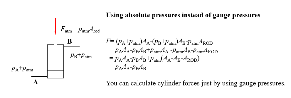
Usage of absolute pressures
Assignment 2 updated (12.2.2019)
Page 13, correction (10.2.2019)0.45 l/min leakage @ 35 bar Þ 0.45 l/min leakage @ 50 barPages 8 and 11 (12.2.2019)New output tables for both loads (m1 and m2)Hints!
1.
Get new inspiration from "calculation exercises".
2.
You can notice "essential similarities" between this assignment (#2) and the Simulink - Simscape assignment. The cases (the systems) are NOT totally the same ("quite or very close") and you can think/ponder what are the differences. However, you can get some inspiration and confidence by examining the Simscape solution if you compare the operation and results.
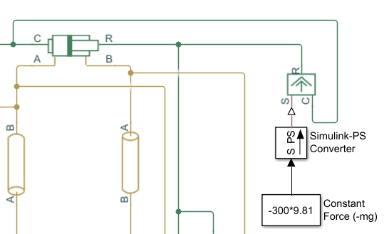
You can add a gravitational load by using for example "Ideal Force Source", "Simulink-PS Converter", and "Constant" blocks to your Simscape application of you want.
It must should be emphasized that the Assignment solution should be carried out by using analytical means, by deriving equations and solving them numerically! Simscape can be used to strengthen your faith and to learn more.
Far below an example of the way the gravitational load (mg) can be added to the cylinder system.
You can find the blocks by a) double clicking Simulink canvas and b) writing part of the block name.
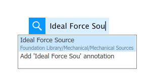
Blocks:
- Ideal Force Source (Foundation Library /Mechanical / Mechanical Sources -library)
- Simulink-PS Converter (Copy - Paste, old design in the figure), and
- Constant (from Sources library)
3.
Remember that
- cylinder is also a pressure transformer (force balance equation)
- cylinder is also a flow rate transformer (continuity equation binding A and B flow rates and piston velocity together)
Create
- Force equation (cylinder)
- Continuity equations (cylinder chamber flows and piston velocity)
Use
- Turbulent throttle equation(s)
- Boundary conditions are pump and tank pressure:
- describe throttle flows as functions of pressures (pressure differences) AND piston velocity
- you can have equation for force balance as a function of
- piston velocity,
- command signal (U), and
- pump pressure.
- Solve for the piston velocity.
- After that you can solve all the other variables.
Other solution methods also possible!
Page 6 (used to be page 5), Inputs•qv_pump pump’s flow rate is adapted for the motion, pressure relief valve is closed!- This value is not given, you have to calculate it.- The text means that the flow rate from pump is the same as the flow rate to cylinder, no flow through PRV.Valve capacity
"valve capacity, full opening (40 l/min @ 35 bar)"
This means that
- with full opening (+/-10 V )
- with 35 bar pressure difference
- 40 l/min flow rate through (one throttle)
-> if you know
- valve command signal
- pressure difference
- you can calculate the flow rate
OR
-> if you know
- valve command signal
- the flow rate
- you can calculate the pressure difference
-
Group Assignment 1 Mailbox
Two documents
- Template with Results
- Calculation file (pdf)
-
Laboratory Assignments - Hydraulics
Read the instructions and perform the Preliminary Task before arriving at the exercise.
-
Comments on Simscape Fluids exercise
Teacher’s overall view is that the students could manage the use of Simulink/Simscape surprisingly well.
The exercise is still new and it will developed according to teacher’s experiences and students’ feedback, which was very welcome.
The ergonomics of Simscape is rather good. Even beginners learn to use it quickly. The challenges are in selection of system parameters. You should know what to component parameters and system inputs to give, otherwise you can get whatever results. The case is similar to usage of other simulators as well. You should know the technology you study and the system characteristics so precisely that you are able to criticize the numerical solutions and you can interpret the results correctly.
Simscape’s challenge/problem is that the sub-models are quite “black boxes”. You no not really know what is happening inside the modules. Mathworks publishes the system equations used in the models but it is hard to know the way the numerical solution is made.
If you make the system model by yourself for example in Simulink environment you should know accurately how the system behaves and what phenomena your system covers … and what phenomena it does not describe.
Therefore also the calculations we have done during the Basics course are important. You should have the intuition and also view based on these basic calculations what kind of operation and numerical results should be expected from the system and its simulation model. You should compare your own, handmade results with the simulation output and be critical.
The position servo we studied works quite fine with only P control. The experiences could be different if we would had a velocity servo under investigation. The integrator which is already in the position servo system takes care that final error is small. However, there is small error left and we could not get rid of it completely. With higher P gain the error is reduced but that will eventually lead to system instability.
The stability problems appear (in this case) as a bounded vibration. In position signal this can be quite difficult to observe. However, if you study the velocity or acceleration outputs this oscillation would be observable more easily. In our model with only inertia (mass) load the cylinder pressure signals (A and B) together determine the acceleration, so the oscillation is also visible in cylinder pressures.
The velocity and displacement signals are integrated or double integrated acceleration signals so those signals are heavily filtered (by integration).
To get rid of the error probably small integrator (I term with small gain) in controller would be needed. High gain would be a stability risk again.
Making the system work “faster” (small rise time) is rather impossible (in this case) with just manipulating controller parameters since during the (fast) movement the proportional control valve is fully open and to get more speed we would need more pressure difference over the valve or a cylinder with smaller piston areas. Higher pressure difference could be realized by raising pump pressure (PRV or pressure compensated pump setting). Also the acceleration phase could be shorter/faster by having more pressure and thus also force.
The overshoot in our case is small or can be absent. The definition in this case is “the ratio of difference between output y’s first maximum and its new steady-state value to its new steady-state value”. To be very precise we should compare the “first maximum” and the “new steady state value” which in our case is not exactly the command value because of steady state error. However, the steady state error is only about 1 mm, so the numerical “error in overshoot value” is not very meaningful.
The 95% rise time used (time it takes for the response to rise from zero to 95% of the steady-state response) is probably not as practical as 5-95% or 10-90% would be. In our simulated case the numerical noise is very small but in practical systems it can be significant so it could be more functional to use a criteria which does not start from zero. In systems with noise it can be difficult to identify when the variable is “in zero”.
Settling time (the time that after a stepwise change in system’s setting value w is required for the process output y to reach and remain inside a band whose width is equal to ±5% of the total change in y, sometimes also other bandwidths are used, e.g., ±1 %, ±2 %) in our studied case was (about) the same as the rise time because the signal never got out of the ±5% “pipe” after it had entered it.
The teacher is happy with the students’ results. Encouraged by this year’s experiences this exercise will be further developed and used in a new and hopefully enhanced form the next year.
-
-
-
-
-
Group Assignment 2 Mailbox
Two documents
- Template with Results
- Calculation file (pdf)
-
-
Group Assignment 3 Mailbox
Two documents
- Template with Results
- Calculation file with derived equations shown (pdf)
-
Simscape assignment
Simscape assignment
4 Exercises for this assignment
1. Monday 3.2.2020 at 12.00 o'clockMaariCD
2. Thursday 6.2.2020 at 14.00 o'clock MaariCD
3. Monday 10.2.2020 at 12.00 o'clock MaariCD
4. Thursday 13.2.2020 at 14.00 o'clock MaariCD
Attending at least two (2) sessions will give you Activity points (3 + 3)Documents available
- Instructions (Word)
- Report file (Powerpoint)
Students' outputs
- Report file, filled (Powerpoint)
- Simulation model (final, closed loop controlled system)
Deadline 6.3.2020
-