
WAT-E2090 - Water and People in a Changing World D, Lecture, 25.10.2022-1.12.2022
This course space end date is set to 01.12.2022 Search Courses: WAT-E2090
Topic outline
-
Guides to R and some of the most common packages
- Introduction to R (html)
- R cheat sheet (pdf)
- ggplot2 website containing full reference, cheatsheet, and links to tutorials (html)
- mapping with tmap (html)
- Scico color package (html)
- Various other R package cheat sheets provided by RStudio (html/pdf)
- R graph gallery (lot of example codes to produce different kind of graphs)
Git• Quick Git guide and a cheatsheet
During this course, we're applying only a fraction of Git features. If you want to dive further into using Git, see the guide above for a rather comprehensive quick-tutorial. While the use Git is not in the center in the learning outcomes of the course, it is a very valuable and useful tool to get a grip on.
Support
• The easiest is to google the command or task you want to do; there is lots of help in the web (including stackoverflow, various R mailing lists etc.).
• R has a strong community around it since it's open source; most likely, someone else has had similar issues than you are having and has asked about it in some forums.
• ?function (e.g. ?mean) in R console will open a help page.
• Posting to Teams Discussion channel - optimally very efficient and enables learning together with your peers!
• Naturally, the teachers will help you when needed
Extra data related to the data introduced in hands-on sessions - all files are in data folder
Week 1:
- Historical runoff, precipitation and temperature data (Data/climate/historical and Data/runoff). Two-decade averages of monthly values for timesteps 1960-1979, 1980-1999, and 2000-2018 (2000-2014 for runoff).
- Future precipitation and temperature data (Data/climate/future). Two-decade averages of 2041-2060; monthly and annual values for scenarios SSP1-RCP2.6 and SSP3-RCP7.0. More on SSPs & RCPs.
Week 2:
- Future total population for scenarios SSP1 and SSP3; years 2050 and 2100 (Data/population).
- Built-up area defined as "artificial areas contiguously occupied by humans (therefore not including vegetative land cover and water, nor roads)", as fractions of cell area. See HYDE 3.1 for description.
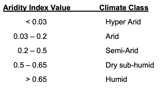
- Aridity class and aridity index (Data/misc). Thresholds from source Table 2.
- Distance to nearest freshwater feature and distance to nearest sea (dist2water and dist2sea; Data/misc)
- Ground elevation (Data/misc)
- Groundwater table depth, annual long-term average (Data/misc)
Week 3:
- Food crop production (kcal) in 2010 as raster, Data/food_prod/crop_production_kcal_2010_025dgr.tif.
- Food supply (kcal/cap/d) in Data/food_prod/food_supply.xlsx. The food supply quantity presented here is based on a national balance of total food supply = production + imports - exports + changes in stocks for all food items in FAOSTAT. From the total supply, the shares of usage for feed, seed, manufacturing for both food and non-food products, and losses during storage and transportation are subtracted before finally yielding the total food supply available for human consumption. Hence, this food supply represents the amount of calories available for human consumption, but not necessarily the amount ending up consumed as retail and household losses are not accounted for.
- BMI (body mass index) data from NCD-RisC (http://www.ncdrisc.org/) including mean BMI as well as share of population overweight and obese: Data/food_prod/NCD_RisC_Lancet_2017_BMI.xlsx.
Week 4:- Environmental flow requirements (EFR) in Data/wateruse/EFR_fraction_annual_1971_2010.tif. This describes the fraction of discharge/runoff used by the natural environment. If the EFR is fulfilled, the riverine ecosystems assumed to be in a fair condition. The values are computed from long-term runoff (1970-2000) as annual averages using the variable monthly flow (VMF) method described in Pastor et al. (2014).
Week 5:
- No specific extra data for this week.
Week 6:
- No specific extra data for this week. Most of the indicators included in the demo code have one additional timestep, which can be taken advantage of.