
CHEM-E4106 - Electrochemistry D, Lecture, 10.1.2022-22.2.2022
This course space end date is set to 22.02.2022 Search Courses: CHEM-E4106
Kirja
5. Electrical double layer and adsorption
5.3. Gouy-Chapman model
The classic Gouy-Chapman model describes the layer between the outer
Helmholtz plane and the bulk of the solution. In this layer, the charges are
assumed to be point charges and the solution is a medium without a structure
described by the relative permittivity  r. Since the only thing that matters is the potential difference, the
potential of the bulk solution can be assumed to be zero and the potential of the
Helmholtz plane is denoted
r. Since the only thing that matters is the potential difference, the
potential of the bulk solution can be assumed to be zero and the potential of the
Helmholtz plane is denoted  2. Let us leave the inner layer for a moment and
take a closer look at the diffuse layer.
2. Let us leave the inner layer for a moment and
take a closer look at the diffuse layer.
The total charge density  (x) is obtained from
electrostatics using the Poisson equation:
(x) is obtained from
electrostatics using the Poisson equation:
=-\varepsilon_r\varepsilon_0\frac{d^2\phi}{dx^2}") |
(5.33) |
|---|
On the other hand, the charge density can be expressed as the sum of all ions present in the diffuse layer:
=\sum_iz_iFc_i(x)") |
(5.34) |
|---|
The ions in the double layer follow the Boltzmann distribution:
=c_i^b\exp\left(-\frac{z_iF\phi}{RT}\right)") |
(5.35) |
|---|
Combing the two equations, we get the Poisson-Boltzmann differential equation:
") |
(5.36) |
|---|
Intergration by substitution gives
 |
(5.37) |
|---|
Thus
d\phi") |
(5.38) |
^2=\frac{RT}{\varepsilon_r\varepsilon_0}\sum\limits_iz_ic_i^b\exp\left(-\frac{z_iF\phi}{RT}\right)+B") |
(5.39) |
|---|
The integration constant B can be determined with the help of the following boundary
conditions: The electric field must vanish in the bulk solution, and thus this
symmetry requirement results in a boundary condition d/dx = 0. According to
the electroneutrality condition, the net charge of the bulk must also be zero, and therefore
= 0. Equation (5.39) therefore becomes
![\displaystyle\frac{1}{2}\left(\frac{d\phi}{dx}\right)^2=\frac{RT}{\varepsilon_r\varepsilon_0}\sum\limits_iz_ic_i^b\left[\exp\left(-\frac{z_iF\phi}{RT}\right)-1\right]](https://mycourses.aalto.fi/filter/tex/pix.php/a0268db5355031bfc5dc9ba47e068554.gif "\displaystyle\frac{1}{2}\left(\frac{d\phi}{dx}\right)^2=\frac{RT}{\varepsilon_r\varepsilon_0}\sum\limits_iz_ic_i^b\left[\exp\left(-\frac{z_iF\phi}{RT}\right)-1\right]") |
(5.40) |
|---|
Consider a symmetrical electrolyte, e.g. NaCl (1:1) or CaCO3 (2:2). Equation (5.40) becomes now
![\displaystyle\left(\frac{d\phi}{dx}\right)^2=\frac{2RTc^b}{\varepsilon_r\varepsilon_0}\left[\exp\left(\frac{-zF\phi}{RT}\right)+\exp\left(\frac{zF\phi}{RT}\right)-2\right]=\frac{8RTc^b}{\varepsilon_r\varepsilon_0}\sinh^2\left(\frac{zF\phi}{2RT}\right)](https://mycourses.aalto.fi/filter/tex/pix.php/02c284b523806773ba0ce7f0c54b1828.gif "\displaystyle\left(\frac{d\phi}{dx}\right)^2=\frac{2RTc^b}{\varepsilon_r\varepsilon_0}\left[\exp\left(\frac{-zF\phi}{RT}\right)+\exp\left(\frac{zF\phi}{RT}\right)-2\right]=\frac{8RTc^b}{\varepsilon_r\varepsilon_0}\sinh^2\left(\frac{zF\phi}{2RT}\right)") |
(5.41) |
^{1/2}\sinh\left(\frac{zF\phi}{2RT}\right)") |
(5.42) |
|---|
Note that we need to choose the negative root
for (ddx)! The equation can be
integrated in a closed form, and after some slightly tedious algebra, the
solution becomes
}{\tanh(zF\phi_0/4RT)}=\exp(-\kappa x)") |
(5.43) |
|---|
where 0 is
potential at the electrode surface (x
= 0) and
^{1/2}") |
(5.44) |
|---|
is again the Debye length (see also Equation (2.33)). The potential profile (5.43) is not very illustrative and because of that, the tanh terms are usually linearized, tanh(x) ≈ x. The linearized result is simply
=\phi_0e^{-\kappa x}") |
(5.45) |
|---|
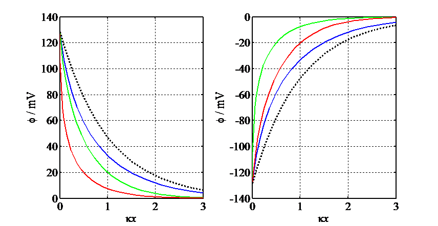
Figure 5.4. Simulated
potential profiles according to Gouy-Chapman theory, F0/RT = ±5: 1:1 electrolyte (blue), 2:1 electrolyte (green), 1:2
electrolyte (red). The black broken line describes the linearized equation (5.44).
When 0 > 0, the curve for the 2:2 electrolyte
almost merges with the curve for the 1:2 electrolyte (red) and when 0 < 0, the
curve for the 2:1 electrolyte (green). Note the order of the curves with
respect to 0.
The potential profiles are shown in Figure 5.4, including for the unsymmetrical electrolytes obtained by integrating Equation (5.40)
numerically. In Figure 5.4,  = (2cbF2/r0RT)1/2.
In aqueous solution at 25 ºC, the Debye length is
–1 ≈ 10–9 (z2cb)–1/2(mol/cm)1/2.
A good rule of thumb is that in 1.0 mM solution, for 1:1 electrolyte –1 ≈ 10 nm.
According to Gauss's law, the charge q inside the volume V is
 |
(5.46) |
|---|
where E
is the electric field through a surface S.
In our one-dimensional case, the scalar product E·dS is zero at all points except on the electrode surface, where it is (d/dx)0dS. The charge density of the double layer is therefore
_0") |
(5.47) |
|---|
The charge density of the electrode for a symmetrical electrolyte is
^{1/2}\sinh\left(\frac{zF\phi_0}{2RT}\right)") |
(5.48) |
|---|
The differential capacitance of the electrode therefore becomes
^{1/2}\cosh\left(\frac{zF\phi_0}{2RT}\right)") |
(5.49) |
|---|
The scaled differential capacitances are shown in Figure 5.5, including for the unsymmetrical electrolytes. Even though the potential profiles cannot be determined in a closed form, the capacitances can be calculated using Equations (5.40) and (5.47).
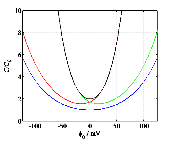
Figure 5.5. Simulated capacitances according to Gouy-Chapman theory: 1:1 electrolyte (blue), 2:1 electrolyte (green), 1:2 electrolyte (red), 2:2 electrolyte (black).
The scaled capacitances for 1:1 electrolytes are:
") |
(5.50a) |
|---|
For a 2:1 electrolyte:
 |
(5.50b) |
|---|
For a 1:2 electrolyte:
 |
(5.50c) |
|---|
And for a 2:2 electrolyte:
") |
(5.50d) |
^{1/2}") ; ;  |
(5.51) |
|---|