CHEM-E4185 - Electrochemical Kinetics, 25.02.2019-29.05.2019
This course space end date is set to 29.05.2019 Search Courses: CHEM-E4185
Kirja
2. Thermodynamics of electrolyte solutions
2.5. Ion-ion interactions
2.5.1 Mean activity coefficient
Activity coefficients of non-electrolytes are close to unity even at moderately concentrated solutions while long-range electrostatic forces between ions mean the activity coefficients of ions must be taken into account even at rather dilute concentrations (c > 1 mM). Ion-ion interaction is traditionally estimated using the Debye-Hückel theory whereby the solvent is taken as a dielectric continuum with a single static relative permittivity \( \varepsilon \)r.
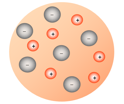
Around an arbitrarily chosen central ion there are more ions with an opposite charge than ions with a like charge.
Ions are arranged in the electric field of the central ion according to the Boltzmann distribution:
| \( \displaystyle c_i(r)=c_i^be^{-z_i \phi (r)} \) | (2.31) |
|---|
ci is the concentration of ion i and \( \varphi=F\phi/RT \). Far from the central ion \( \varphi \)(r) = 0, hence ci has its bulk value \( c_i^b \). The charge density \( \rho \)(r) around the central ion is
| \( \displaystyle\rho(r)=\sum\limits_{i}z_iFc_i=\sum\limits_{i}z_iFc_i^be^{-z_i\phi(r)} \approx \sum\limits_{i}z_iFc_i^b\left(1- \frac{z_iF\phi(r)}{RT}\right) =- \frac{F^2\phi(r)}{RT}\sum\limits_{i}z_i^2c_i^b \) | (2.32) |
|---|
It can be shown that the linearization of the exponent is acceptable when c < 0.01 mol/dm3 (T = 298); the last equality comes from electroneutrality in the bulk phase. Inserting the charge density into Poisson equation gives
| \( \displaystyle\nabla^2\phi=- \frac{\rho}{\varepsilon_0\varepsilon_r} \Rightarrow \nabla^2\phi=\kappa^2\phi \) ; \( \kappa^2 \frac{F^2}{\varepsilon_0\varepsilon_rRT}\sum\limits_{i}z_i^2c_i^b \) | (2.33) |
|---|
The quantity \( \kappa \)-1 is known as the Debye length because it bears the length unit. It is a characteristic measure of the thickness of the electric double layer (EDL, Chapter 5), in other words the distance where local electroneutrality does not apply. In an aqueous solution of a 1:1 electrolyte at the 1.0 mM concentration it takes the value of approximately 10 nm (T = 298 K).
The solution of Equation (2.33) in spherical coordinate is (φ(r) = 0 when r → ∞)
| \( \displaystyle r\phi(r)=Ce^{-\kappa r} \) | (2.34) |
|---|
The constant C is solved from the condition that the ion cloud around the central ions compensates its charge zce:
| \( \displaystyle \int_{a}^{\infty }{4\pi r^2\rho(r)dr=-z_ce} \) , | (2.35) |
|---|
Here, a is the distance
of closest approach to the central ion. Using straightforward algebra, the constant C and the potential distribution is obtained as
| \( \displaystyle C=\frac{z_ce} {4\pi\varepsilon_0 \varepsilon_r }\frac{e^{\kappa a}}{1+\kappa a} \Rightarrow \phi(r)=\frac{z_ce} {4\pi\varepsilon_0 \varepsilon_r }\frac{e^{-\kappa(r-a)}}{1+\kappa a}\frac{1}{r} \) | (2.36) |
|---|
Figure 2.3. Scaled potential e−κr as the function of the distance from the central ion at varying concentrations (1-100 mM) of a 1:1 electrolyte; central ion assumed a point charge, a = 0.
In Figure 2.3 above, the potential profiles have been shown as the function of the distance from the central ion. The reference value is the potential created by a single ion
| \( \displaystyle V(r)=\frac{z_ce}{4\pi\varepsilon_0\varepsilon_r}\frac{1}{r} \) | (2.37) |
|---|
The electrostatic work required to bring the central ion into the ion cloud is
| \( \displaystyle w_{\text{ion-ion}}=N_A \int_{0}^{z_ce}{\phi_{\text{atm}}} (a)dq \) ; \( \phi_{\text{atm}}(a)=\phi (a)-V(a)=-\frac{z_ce}{4\pi\varepsilon_0\varepsilon_r}\frac{\kappa}{1+\kappa a}\) | (2.38) |
|---|
| \( \displaystyle w_{\text{ion-ion}}=-\frac{N_A\kappa}{8\pi\varepsilon_0\varepsilon_r}\frac{{(z_ce)^2}}{1+\kappa a} \) | (2.39) |
|---|
When a solution is diluted from concentration c1 to concentration c2, the work of dilution is
| \( \displaystyle w_{\text{dil}}=RT\ln(\frac{a_2}{a_1})=RT\ln(\frac{c_2}{c_1})+RT\ln(\frac{\gamma_1}{\gamma_2})=w_{\text{osm}}+w_{\text{el}} \) | (2.40) |
|---|
Assuming that electrostatic interactions is the root of an activity coefficient, the latter term in the above equation is equal to wion-ion. Since γ2 = 1 (assuming infinite dilution)
| \(\displaystyle \ln\gamma_i=\frac{w_{\text{ion-ion}}}{RT}=-\frac{(z_ce)^2}{8\pi\varepsilon_0\varepsilon_rk_BT}\frac{\kappa}{1+\kappa a} \) | (2.41) |
|---|
It is customary to write Equation (2.41) down with the Briggs logarithm:
| \( \displaystyle\log\gamma_i=-z_i^2\frac{A\sqrt{I}}{1+Ba\sqrt{I}} \) ; \( I=\frac{1}{2}\sum\limits_{i}z_i^2c_i= \) ionic strength | (2.42) |
|---|
\( \displaystyle A= \frac{1.8246 \cdot10^6 }{(\varepsilon_rT)^{3/2}} \) mol-1/2dm3/2K3/2 ; \( \displaystyle B=\frac{50.29 \cdot10^8}{(\varepsilon_rT)^{1/2}} \) cm-1dm3/2K1/2
Applying the definition of the mean activity coefficient (2.16) the following result is reached:
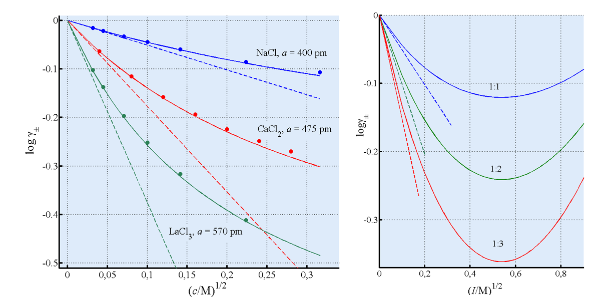
| \( \displaystyle\log\gamma_{\pm}=z_+z_-\frac{A\sqrt{I}}{1+Ba\sqrt{I}} \) | (2.43) |
|---|
The parameter a is known as the distance of closest approach, the minimum distance between a cation and an anion. In aqueous solutions, the Debye-Hückel model works satisfactorily up to a concentration of 0.1 M. Often only the numerator of Equation (2.43) is used (Debye-Hückel limiting law) if c < 0.01 M. Various more or less empirical equations have been suggested for more concentrated solutions; perhaps the best known is the Davies formula that takes the following form for aqueous solutions at 298 K:
| \( \displaystyle\log\gamma_{\pm}=z_+z_-\frac{0.51\sqrt{I}}{1+\sqrt{I}}-0.20I \) | (2.44) |
|---|
2.5.2 Ion pairing
In solvents with low relative permittivity, ions tend to form ion pairs. Although an electrolyte might dissolve completely in the solvent, it does not dissociate completely into free ions. Dissociation constants can be determined experimentally using, for example, conductivity measurements. The dissociation constant of an electrolyte \( \text{A}_{\upsilon+}B_{\upsilon-} \) , Kd is
| \( \displaystyle K_d=\frac{(\gamma_Ac_A)^{\upsilon_+}(\gamma_Bc_B)^{ \upsilon_-}}{c_{AB}}=\frac{(\alpha\gamma_{\pm})^{\upsilon}c^{\upsilon-1}}{1-\alpha} \) | (2.45) |
|---|
where \( \alpha \) is the degree of dissociation and \( \upsilon=\upsilon_++\upsilon_- \) The activity coefficient of ion pairs is usually taken as unity because they carry no charge. Since α often is rather low, making the ionic strength also low, the mean activity coefficient \( \gamma_{\pm} \) is close to unity. In that case, for a 1:1 electrolyte applies Kd = α2c/(1 - α).
Ion pairing (or ion association) is traditionally analyzed using the theories of Bjerrum or Fuoss. The Bjerrum theory assumes that close to an ion the potential profile is essentially V(r), Equation (2.37). The number of ions i residing in the sphere element of the thickness of dr is therefore
| \( \displaystyle dN_i(r)=4\pi r^2N_i^b\exp(-\frac{z_ieV}{k_BT})dr=4\pi r^2N_i^b\exp(-\frac{z_iz_ce^2}{4\pi\varepsilon_0\varepsilon_rk_BT}\frac{1}{r})dr \) | (2.46) |
|---|
Function (2.46) has a minimum at the point
| \( \displaystyle r=q=\displaystyle\frac{|{z_iz_c|}e^2}{8\pi\varepsilon_0\varepsilon_rk_BT} \) | (2.47) |
|---|
Bjerrum postulated that all ions with the sign opposite to that of the central ion within a distance smaller than q form an ion pair. At the distance q the electrostatic energy of an ion is
| \( \displaystyle\frac{|{z_iz_c|}e^2}{4\pi\varepsilon_0\varepsilon_rq}=2k_BT \) | (2.48) |
|---|
The fraction of paired (associated) ions, 1 - α, is therefore
| \( \displaystyle 1-\alpha= \int_{a}^{q}{dN_i(r)dr} =4\pi N_i^b \int_{a}^{q}{r^2e^{2q/r}dr} \) | (2.49) |
|---|
With the change of variables x = 2q/r the above equation can be written in the form of
| \( \displaystyle 1-\alpha=4\pi N_i^b \cdot(2q)^3 \int_{2}^{b}{x^{-4}e^xdx} \) ; \( b=\frac{2q}{a}=\frac{|{z_+z_-|}e^2}{4\pi\varepsilon_0\varepsilon_rak_BT} \) | (2.50) |
|---|
The integral (Bjerrum integral) in the above equation must be evaluated numerically. The ion-pairing (association) constant Ka (= 1/Kd) is relatively easy to calculate. Assume an ion-pairing reaction A+ + B- ↔ AB. Now, from Equation (2.45)
| \( \displaystyle K_a=\frac{1-\alpha}{\alpha^2c}\frac{\gamma_{\text{AB}}}{\gamma_{\pm}^2} \) | (2.51) |
|---|
Because Ka is the same at each concentration, in a very diluted solution where α ≈ 1 and \( \gamma_{\pm} \) ≈ 1, Ka ≈ (1 - α)/c. Inserting Equation (2.50) into this and changing the species number density Nib (m-3) to the molar concentration gives
| \( \displaystyle K_a=4000\pi N_A(\frac{|{z_iz_c|}e^2}{8\pi\varepsilon_0\varepsilon_rk_BT})^3 \int_{2}^{b}{x^{-4}e^xdx} \) | (2.52) |
|---|
where NA is the Avogadro number, 6.023×10²³ mol-1. The weakest point in the Bjerrum theory is its rather arbitrary choice q = 2kBT. For a 1:1 electrolyte in water at room temperature (298 K) the value of Ka is ca. 1.27 dm3/mol (a = 0.2 nm), proving that common electrolytes do not make ion pairs in water to a significant extent.
The Fuoss theory presumes contact between ions in order to form an ion pair. Let’s consider again a 1:1 electrolyte. Let the number of free ions in the solution be N+ = N- = N1 and N2 the number of ion pairs. After adding δN anions and cations in the solution a fraction of them remains free and a fraction makes ion pairs. The probability that an anion remains free is proportional to the amount of δN added and to the volume that is not occupied by cations:
| P(free) \( \displaystyle \sim(V-N_1 \nu_+) \delta N \) | (2.53) |
|---|
where V
is the total solution volume and ν+
the volume of a cation. Accordingly, the probability that an anion makes an ion
pair is, in addition to space occupied by cations, N1v+, and to the added amount, δN also proportional to the Boltzmann factor e-E(a)/kBT:*
| P(ion pair) \( \displaystyle \sim N_1\nu_+e^{-E(a)/k_BT} \delta N \) | (2.54) |
|---|
The electrostatic energy of an anion in contact with a cation, E(a) is obtained from Equation (2.37). Let the number of anions that make an ion pair be δN2 and the number of anions remaining free δN1. A similar analysis can of course be done for cations. Due to electroneutrality, the number of cations that make ion pairs must also be δN2, making the total number ion pairs 2δN2. Probabilities are proportional to the numbers. Therefore,
| \( \displaystyle\frac{\delta N_2}{\delta N_1}=\frac{2N_1 \nu_+e^{-E(a)/k_BT}dN}{(V-N_1 \nu_+)dN } \) | (2.55) |
|---|
Assuming that the solution is so dilute that the volume occupied by cations, N1v+, is insignificant with respect to the solution volume V, Equation (2.55) can be integrated with respect to N1. The result is of course
| \( \displaystyle N_2=N_1^2e^{E(a)/k_BT}\nu_ +/V \) | (2.56) |
|---|
The concentration of free ions, N1/V, is in terms of molarity
| \( \displaystyle N_1/V= \alpha cN_A \cdot1000 \) | (2.57) |
|---|
Accordingly, the concentration of ion pairs is
| \( \displaystyle N_2/V=(N_1/V)^2e^{-E(a)/k_BT}(4/3)\pi a^3=(1- \alpha)cN_A \cdot1000 \) | (2.58) |
|---|
Combining Equations (2.51), (2.57) and (2.58) the following formula is reached:
| \( \displaystyle\frac{1-\alpha}{\alpha^2c}=1000N_A(\frac{4}{3}\pi a^3)e^{-E(a)/k_BT} \) | (2.59) |
|---|
The mean activity coefficient is again assumed to be unity due to the dilute concentration.
2.5.3 Super acids and Hammett acid function[1]
In very strong acids, such as in pure sulphuric acid or in its mixtures with organic solvents, ion association and activity coefficients become rather ambiguous quantities. Yet it has been experimentally demonstrated that these kinds of solutions are very acidic, having a negative pH: they are called super acids. Analogously, mixtures of strong bases with organic solvents are vary basic, having a pH beyond the scale of ordinary pH sensors because they can make the sensor unstable or even destroy it.
For the analysis of super acids and bases, Hammett introduced an acid function H0 that can be considered to be an extension of the common pH scale. In order to determine the value of H0, a weak indicator base B is added to the super acid solution, and the concentration of B is determined with, for example, UV spectrophotometer. The base protonates to BH+, and its dissociation equilibrium is
| BH+ \(\ce{ <=> }\) B + H+ | (2.60) |
|---|
The equilibrium constant is of course
| \( \displaystyle K_d=\frac{a_{H^+}a_B}{a_{BH^+}} \) | (2.61) |
|---|
Taking the negative of the Briggs logarithm as usual
| \( \displaystyle pK_d+\log\frac{[B]}{[BH^+]}=-\log(a_{H^+})-\log\frac{\gamma_B}{\gamma_{BH^+}} \equiv H_0 \) | (2.62) |
|---|
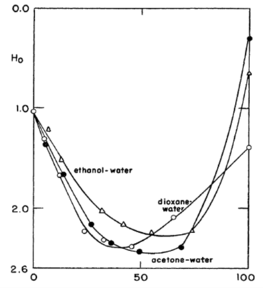
Equation (2.62) defines the Hammett acid function H0 that can be experimentally defined because the concentration ratio [B]/[BH+] can be measured with spectroscopy. For example, for water-free suphuric acid H0 = -12.0. Nitroanilines are typical indicator bases. The values of their equilibrium constants (Kd) in solvents other than water pose a problem of its own that must be solved with various means of comparison and extrapolation6.
In alkaline solutions the corresponding function is H− that corresponds to the equilibrium
| BH + OH−(H2O)n \(\ce{ <=> }\) B− + (n + 1)H2O ; | (2.63) |
|---|
where n is the hydration number of the hydroxide ion. In pure water its value is approximately 5.5. In aqueous solutions the function H− can be estimated with the equation
| \( H_-=pK^w+\log[OH^-]-(n+1)\log[H_2O] \) | (2.64) |
|---|
In Equation (2.64), Kw is the ionic product of water and [H2O] is the concentration of free water in the solution. Their values naturally depend on the solution composition.
* When an anion approaches a cation E(a) is the energy released in the process. The Boltzmann factor is also found in the Grand Canonical partition function of ion binding.
[1] M.A. Paul, F.A. Long, ’H0 and related indicator acidity functions’, Chem. Rev. 57 (1957) 1-45.