CHEM-E4185 - Electrochemical Kinetics, 25.02.2019-29.05.2019
This course space end date is set to 29.05.2019 Search Courses: CHEM-E4185
Kirja
6. Electrochemical reaction kinetics
6.8. Marcus theory
In 1992, Rudolf Marcus received the Nobel Prize in Chemistry for the theory of electron transfer that is commonly known as the Marcus theory. Its predecessors are the studies by Levich [1] and Dogonadze [2] about the reorganization of solvent molecules during a redox reaction. The approach taken by Marcus is based on statistical mechanics, considering the configurations of all molecules participating in the reaction. Each molecule is described as a harmonic oscillator, with an energy that depends in a parabolic manner on the deflection from its equilibrium position. As there are several molecules, each having several modes of vibration, a multi-dimensional energy space is obtained that is very difficult to visualize. We simplify the situation to the two-dimensional Figure 6.12. This approach [3] is closer to the models of Levich and Dogonadze, but is simpler than the accurate treatise by Marcus yet gives the same results.
On the right of Figure 6.11 the free energy profile of the oxidized species ’ox’ is seen. At configuration xox its free energy is Gox. Similarly, the reduced species’red’ has its energy profile on the left: its free energy at configuration xred is Gred. In this simple model, the reaction coordinate can be interpreted as the stretch of the molecular bond from its equilibrium length. The energy profiles intersect at configuration xc, where an electron is transferred from red to ox in an adiabatic process.
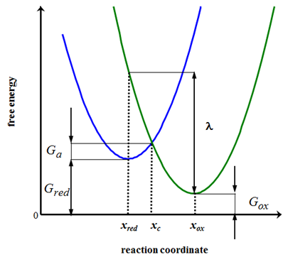
Let’s calculate the abscissa of the intersection of the parabolas, xc:
| \( \displaystyle G_{ox}^c=G_{ox}+\frac{1}{2}h\nu(c_x-x_{ox})^2=G_{red}+\frac{1}{2}h\nu(c_x-x_{red})^2=G_{red}^c \) | (6.111) |
|---|
| \( \displaystyle x_c=\frac{1}{2}(x_{ox}-x_{red})+\frac{\Delta G}{h\nu(x_{ox}-x_{red})} \) ; \( \Delta G=G_{ox}-G_{red} \) |
(6.112) |
|---|
Note that \( \Delta G<0 \). The factor \( h\nu \) is the energy of the fundamental vibration of a harmonic oscillator that is obtained from its quantum mechanical solution; h is the Planck constant, 6.626×10⁻³⁴ Js and \( \nu \) is the vibration frequency (s–1). Inserting the expression of xc into that of Gred, the height of the energy barrier (activation energy) is found to be
| \( \displaystyle\Delta G_a=G_{red}^c-G_{red}=\frac{(\lambda+\Delta G)^2}{4\lambda} \) |
(6.113) |
|---|
| \( \displaystyle\lambda=\frac{1}{2}h\nu(x_{ox}-x_{red})^2 \) | (6.114) |
|---|
The quantity \( \lambda \) is known as the reorganization energy, because it represents the energy change when moving along either of the parabolas between the points xred and xox, i.e. the change in the molecular configuration without electron transfer. It is always a positive quantity.
The rate constant of the reaction is expressed via the theory of activated complexes (absolute rate theory):
| \( \displaystyle k=\frac{k_{\text{B}}T}{h}\kappa e^{-\Delta G_a/RT}=k'e^{-\Delta G_a/RT} \) | (6.115) |
|---|
kB is the Boltzmann constant (1.38×10⁻²³ J K–1) and \( \kappa \) is what is known as transmission coefficient, which is unity for an adiabatic reaction. When the electrode potential is changed, this changes \( \Delta G \) as discussed earlier in this chapter. The charge transfer coefficient \( \alpha \) is therefore found to be
| \( \displaystyle\alpha=\frac{RT}{F}\frac{\partial\text{ln }k}{\partial E}=-\frac{1}{F}\frac{\partial\Delta G_a}{\partial E}=-\frac{1}{2F}\left(1+\frac{\Delta G}{\lambda}\right)\frac{\partial\Delta G}{\partial E}=\frac{1}{2}\left(1+\frac{\Delta G}{\lambda}\right) \) | (6.116) |
|---|
because
| \( \displaystyle\Delta G =-F(E-E^0) \) | (6.117) |
|---|
Thus, if \( \lambda \gg\Delta G \), \( \alpha \approx0.5 \), as is usually found to be the case in experiments in the vicinity of an equilibrium potential. When \( \Delta G \) is increased, the intercept xc approaches the point xred whence\( \Delta G=-\lambda \), Ga = 0 and \( \alpha=0 \). When the intercept xc moves to the left side of xred, Ga starts to increase again, i.e. the reaction rate begins to decrease. This range of potentials is known as the inverted region; its existence was not verified until 1990s. If \( \Delta G>0 \), i.e. the parabola of the species ox is raised with respect to that of the species red, the activation energy increases and \( \alpha \) ultimately approaches unity (\( \Delta G=\lambda \)).
The discussion above covers the reaction ’from left to right’. Considering the inverse reaction ‘from right to left’, it is seen from Figure 6.12 that the activation energy is higher by the amount of \( -\Delta G \). From Equation (6.113) we therefore see that
| \( \displaystyle\Delta G_a'=\Delta G_a-\Delta G=\frac{(\lambda-\Delta G)^2}{4\lambda} \) |
(6.118) |
|---|
We are now able to write down the reaction rate constants as the function of the electrode potential:
| \(\displaystyle k_{ox}=k'\text{exp}\left[-\frac{(\lambda-F(E-E^{0'}))^2}{4\lambda RT}\right] \) | (6.119a) |
| \(\displaystyle k_{red}=k'\text{exp}\left[-\frac{(\lambda+F(E-E^{0'}))^2}{4\lambda RT}\right] \) | (6.119b) |
|---|
Equations (6.119) prove that when E – E0’ increases, the activation energy of oxidation decreases, in other words its reaction rate constant kox increases. Accordingly, the activation energy of reduction increases and kred decreases. It is also evident that at E = E0’
| \(\displaystyle k_{ox}=k_{red}=k'\text{exp}\left[-\frac{\lambda}{RT}\right] \) |
(6.120) |
|---|
The reorganization energy consist of the contributions from the reagents (\( \lambda_i \)) and the solvent (\( \lambda_o \)): \( \lambda=\lambda_i+\lambda_o \). The former includes all the vibration modes of the molecules:
| \(\displaystyle \lambda_i=\sum\limits_k\frac{1}{2}h\nu_k(x-x_k) \) | (6.121) |
|---|
The solvent contribution \( \lambda_o \) comes from the treatise by Marcus, but we can be content with the final result:
| \(\displaystyle \lambda_o=\frac{e^2}{4\pi\varepsilon_0}\left(\frac{1}{r}-\frac{1}{R}\right)\left(\frac{1}{\varepsilon_{opt}}+\frac{1}{\varepsilon_{st}}\right) \) | (6.122) |
|---|
where r is the molecular radius of the reagent and R its distance to the electrode during the reaction; \( \varepsilon_{opt} \) and \( \varepsilon_{st} \) are the optical and static relative permittivity of the solvent*, respectively, e is the elementary charge and \( \varepsilon_0 \) the permittivity of vacuum, 8.854\( \times \)10−12 F/m.
Marcus theory has been further developed (Marcus-Hush, Marcus-Hush-Chidsey theories), but the merit of the original Marcus theory is that it was able to explain the potential dependence of the charge transfer coefficient \( \alpha \) for example, for the first time. It also provides an estimate of the rate constants in different solvents, as shown by Equation (6.122).
You can now test your conceptual knowledge by taking Quiz Chapter 6.
[1] V.G. Levich, Advan. Electrochem. Electrochem. Eng. 4 (1966) 249.
[2] R.R. Dogonadze, (Ed. N.S. Hush), Reactions of molecules at electrodes, Wiley 1971.
[3] Modified from: J. Albery, Electrode kinetics, Clarendon Press, Oxford, 1975.
* Relative permittivity is a complex quantity that has limiting values \( \varepsilon_{opt} \) when \( \omega \) → ∞ and \( \varepsilon_{st} \) when \( \omega \) → 0 where \( \omega \) is the angular frequency of the dielectric measurement; \( \varepsilon_{st} \) is the permittivity that is also known as the dielectric constant (e.g. in water 78.4).