CHEM-E4185 - Electrochemical Kinetics, 25.02.2019-29.05.2019
This course space end date is set to 29.05.2019 Search Courses: CHEM-E4185
Kirja
6. Electrochemical reaction kinetics
6.5. Electrochemical reaction mechanisms
Like all chemical reactions, electrochemical reactions may also consist of several consequtive reaction steps; parallel steps also occur. Reaction mechanisms can be studied with current-voltage curves and in particular with Tafel slopes. The reduction of copper provides a well-known example of a two-step reaction:
| Cu2+ + e- → Cu+ slow | (6.42) |
|---|
| Cu+ + e- → Cu fast | (6.43) |
|---|
The rate constant of the first step has been determined* as \( k_1^0=6.50 \times10^{-5} \text{ cm s}^{-1} \), and that of the second step \( k_2^0=0.139 \text{ cm s}^{-1} \). The second step has also been found to be reversible: the reverse zeroth order reaction rate constant is \( k_{-2}^0=1.88 \times10^{-7} \text {cm}^{-2} \text{s}^{-1} \). Copper is also famous for its disproportionation reaction
| 2 Cu+ → Cu2+ + Cu | (6.44) |
|---|
that has the equilibrium constant of \( 2.20 \times10^{-6} \). As this example shows, an electrochemical reaction can be quite complicated but, like in all reaction kinetics, one step may be rate-determining which simplifies the analysis greatly.
Since the reaction rate is proportional to the electric current, the reaction order, \( \nu_k \), of a species k in the reaction can be determined simply as
| \( \displaystyle\nu_k=\left(\frac{\partial\text{ln}i}{\partial\text{ln}c_k}\right) \) | (6.45) |
|---|
The determination of the reaction order can help in the solving of the reaction mechanism. If the reaction order of a species is zero, for example, it is not part of the electron transfer chain.
6.5.1 Tafel slopes of a two-step reaction
Let’s consider a reaction like that of copper, \(\ce{ R<=>O }\) \( +2\text{ e}^- \) , with the following notation:
| \(\ce{ R <=>[\ce{k_1}][\ce{k_{-1}}] X }\) \( +\text{ e}^- \) | (6.46) |
|---|
| \(\ce{ R <=>[\ce{k_2}][\ce{k_{-2}}] O }\) \( +\text{ e}^- \) | (6.47) |
|---|
The charge transfer coefficient and the formal potential of the first step (6.46) are \( \alpha \) and \( E_1^{0'} \) respectively, and those of the second step (6.47) \( \alpha_2 \) and \( E_2^{0'} \). In the stationary state the reaction rates of steps 1 and 2 are equal, hence d[X]/dt = 0. The total current density is the sum of the currents of the individual steps, i = i1 + i2, therefore i1 = i2 = (1/2)i. Since we are going to derive the Tafel slopes as a function of the rates of the individual reaction steps we consider the potential range where mass transfer is insignificant. Therefore, cR and cO assume their bulk values but the concentration of the intermediate X, cX, depends on the electrode potential. Furthermore, it is assumed that X is not desorbed from the electrode and transported away.
Now we are able to write down the reaction rates in a stationary state:
| \( \displaystyle\frac{1}{2}\frac{i}{F}=\frac{i_1}{F}=k_1^0(c_\text{R}e^{\alpha_1f(E-E^{0'}_1)}-c_\text{X}e^{(\alpha_1-1)f(E-E^{0'}_1)}) \) | (6.48) |
|---|
| \( \displaystyle\frac{1}{2}\frac{i}{F}=\frac{i_2}{F}=k_2^0(c_\text{R}e^{\alpha_2f(E-E^{0'}_2)}-c_\text{O}e^{(\alpha_2-1)f(E-E^{0'}_2)}) \) | (6.49) |
|---|
At equilibrium, the current is zero, i.e. the currents in both steps are zero. At the equilibrium potential, Eeq, the concentration of X is cX,eq. Analogously to Chapter 6.2.2, we can write down the exchange current densities of the reaction steps
| \( \displaystyle i_{0,1}=Fk_1^0(c_{\text{X,eq}})^{\alpha_1}(c_{\text{R}})^{1-\alpha_1} \) |
(6.50) |
|---|
| \( \displaystyle i_{0,2}=Fk_2^0(c_{\text{O}})^{\alpha_2}(c_{\text{X,eq}})^{1-\alpha_2} \) |
(6.51) |
|---|
Current-overpotential equations accordingly become
| \( \displaystyle\frac{i_1}{i_{1,0}}=e^{\alpha_1f\eta}-\left(\frac{c_{\text{X}}}{c_{\text{X,eq}}}\right)e^{(\alpha-1)f\eta} \) |
(6.52) |
|---|
| \( \displaystyle\frac{i_2}{i_{2,0}}=\left(\frac{c_{\text{X}}}{c_{\text{X,eq}}}\right)e^{\alpha_2f\eta}-e^{(\alpha_2-1)f\eta} \) | (6.53) |
|---|
Eliminating (cX/cX,eq) from the above equations, current density is obtained as \( i=2 \cdot i_1=2 \cdot i_2 \):
| \( \displaystyle i=\frac{2(e{^f\eta}-e^{-f\eta})}{(i_{1,0})^{-1}e^{(1-\alpha_1)f\eta}+(i_{2,0})^{-1}e^{-\alpha_2f\eta}} \) | (6.54) |
|---|
When \( f\eta \) » 0, the terms with negative exponential become insignificant, and the anodic Tafel equation is found to be
| \( \displaystyle\eta=\frac{2.303RT}{\alpha_1F}\text{log}(i)-\frac{2.303RT}{\alpha_1F}\text{log}(2i_{1,0}) \) | (6.55) |
|---|
Analogously, when \( f\eta \) « 0, the cathodic Tafel equation is
| \( \displaystyle\eta=\frac{2.303RT}{(\alpha_2-1)F}\text{log}(-i)+\frac{2.303RT}{(1-\alpha_2)F}\text{log}(2i_{2,0}) \) |
(6.56) |
|---|
At sufficiently large overpotentials, the Tafel slopes correspond to one electron transfer, ±118 mV/decade (if \( \alpha_1=\alpha_2=0.5 \)). Extrapolating the Tafel slopes to zero overpotential, i1,0 and i2,0 can be determined. Hence if the intercepts at the current axis are not equal a multi-step mechanism is expected. It is also worth noting that \( \alpha_1+\alpha_2 \) is not necessarily equal to unity.
From Equation (6.54) it is easy to see the effect of the rate-determining step on the Tafel slopes. If i1,0 » i2,0 so the first term in the denominator can be neglected, the anodic Tafel slope is \( \frac{2.303RT}{(1+\alpha_2)F} \), ca. 40 mV/decade if \( \alpha_2=0.5 \). This can be seen in the first curve of Figure 6.6 in the range -2 < log| i/i0,1| < 1; the cathodic Tafel slope follows Equation (6.56). Similarly, if i1,0 « i2,0 the anodic Tafel slope follows Equation (6.55), and the cathodic slope is \( -\frac{2.303RT}{(2-\alpha_1)F} \), the last curve in Figure 6.6 in the range 1 < log| i / i0,1| < 4. At very high overpotentials, Equations (6.55) and (6.56) are valid, as Figure 6.6 also proves. In the case of copper, i1,0 » i2,0, giving the current-overpotential equation
| \( \displaystyle i=2i_{2,0}(e^{(1+\alpha_2)f\eta}-e^{(\alpha_2-1)f\eta}) \) | (6.57) |
|---|
The anodic Tafel slope is approximately 40 mV/decade and the cathodic slope approximately 120 mV/decade, which is experimentally found to be correct.
Another example is the reaction
| Mn4+ + e- → Mn3+ | (6.58) |
|---|
At first glance, the reaction appears to be a simple one-electron transfer, but the concentration of Mn4+ has no effect on current, i.e. its reaction order is zero while the reaction order of Mn3+ is one. The mechanism that explains these results is
| Mn3+ + e- \(\ce{ <=> }\) Mn2+ k1, k-1 | (6.59) |
|---|
| Mn4+ + Mn2+ \(\ce{ <=> }\) 2 Mn3+ k2, k-2 | (6.60) |
|---|
| Mn4+ + e- \(\ce{ <=> }\) Mn3+ | (6.58) |
|---|
Let’s denote [Mn2+] = c1, [Mn3+]
= c2 and [Mn4+] = c3. In
the cathodic potential range, the inverse reaction of (6.59) can be neglected. Making
the steady-state approximation of Mn2+ which does not appear in the
net reaction
| \( \displaystyle\frac{dc_1}{dt}=k_1c_2-k_2c_1c_3+k_{-2}c_2^2=0 \Rightarrow \nu=-\frac{dc_3}{dt}=k_2c_1c_3-k_{-2}c_2^2=k_1c_2 \) | (6.61) |
|---|
Equation (6.61) confirms that the reaction is of the first order with respect to Mn3+ and of the zeroth order with respect to Mn4+. Since the disproportionation reaction (6.60) does not include electron transfer, the concentration of Mn4+ does not contribute to electric current; the reaction therefore represents an EC mechanism.
If reaction (6.60) were rate-determining, Mn2+ would accumulate to such a large extent that the inverse reaction of (6.59) should also be taken into account. In general, reactions preceding the rate-determining step stay at equilibrium and, therefore, c1 = K1c2 where K1 would be the equilibrium constant of reaction (6.59). This would convert Equation (6.61) into the form of (k-2 = 0)
| \( \displaystyle\nu=-\frac{dc_3}{dt}=k_2K_1c_2c_3 \) | (6.62) |
|---|
The net reaction would therefore be of the first order with respect to both Mn3+ and Mn4+. As K1 is a function of the electrode potential† according to the Nernst equation and k2 is independent of potential, the Tafel slope would be 59 mV/decade.
Finally, let’s compare the following mechanisms semi-qualitatively:
| A +
e-\(\ce{ <=>[\ce{k_1}] }\) B
+ e- \(\ce{ ->[\ce{k_2}] }\) C |
(6.63) |
|---|
| \( \displaystyle\begin{cases}\text{A}+\text{e}^- \rightarrow \text{B}\text{, }k_1 \\\text{A}+\text{e}^- \rightarrow \text{C}\text{, }k_2\end{cases} \) | (6.64) |
|---|
If the first step of the consequtive reaction mechanism (6.63) is rate-determining, as soon as B is formed, it reacts further to C. Since both steps include electron transfer, the total current is i = 2·i1, but the Tafel slope is determined from the first step. If the second step is rate-determining, i = 2·i2 and the Tafel slope is \( -\frac{2.303RT}{(2-\alpha_2)F} \) because
| \( -\displaystyle\frac{i_2}{F}=[B]k_2^0e^{(\alpha_2-1)f(E-E_2^{0'})}=[A]e^{-f(E-E_1^{0'})}k_2^0e^{(\alpha_2-1)f(E-E_2^{0'})}=[A]e^{-f(E_2^{0'}-E_1^{0'})}k_2^0e^{-f(2-\alpha_2)(E-E_2^{0'})}=\text{constant} \cdot e^{f(\alpha_2-2)(E-E_2^{0'})} \) | (6.65) |
|---|
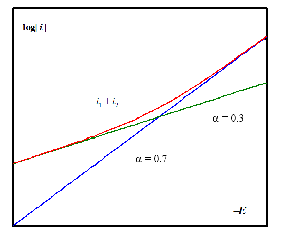
The analysis of parallel reactions (6.64) is easier: i = i1 + i2 and the Tafel slope is determined by the faster reaction. If \( \alpha_1 \) and \( \alpha_2 \) are significantly different, the Tafel slope may vary because the rates of the individual reactions vary at a different pace as a function of the electrode potential. In Figure 6.7, at low electrode potentials the first reaction with higher exchange current density i0,1 and \( \alpha_1=0.3 \) controls current, but at higher electrode potentials the other reaction with lower exchange current density i0,2 and \( \alpha_2=0.7 \) takes control because the exponential function overcomes the difference in exchange current densities.
6.5.2 Hydrogen evolution
Hydrogen evolution is probably the most studied electrochemical reaction due to its immense industrial significance. In the electrolytic production of metals, for example, hydrogen evolution defines the upper limit of the cathodic overpotential that can be used; this issue was discussed in Chapter 4 in connection with Pourbaix diagrams. Splitting water into hydrogen and oxygen in an electrolyzer is another application that may be particularly important in hydrogen economy in the future, see Chapter XX. Furthermore, the inverse reaction of hydrogen evolution, the catalytic dissociation of hydrogen to protons and electrons, is the core reaction in the hydrogen fuel cell.
The rate of hydrogen evolution very much depends on the electrode material, because the reaction includes an adsorption step as described below. The ability of a metal to facilitate hydrogen evolution is illustrated in the volcano plot, Figure 6.8.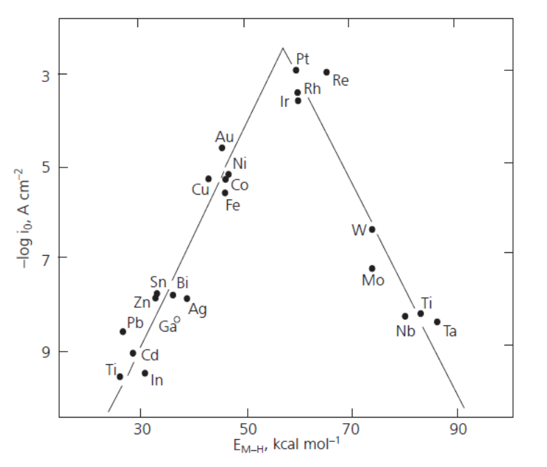
Figure 6.8. Volcano plot: The dependence of the exchange current density of the hydrogen evolution reaction on the adsorption enthalpy of hydrogen. From: Holton et al., Platinum Metals Review, 57 (2013) 259-271 (with publisher’s permission).
The volcano plot is represented in various ways in the literature, but its interpretation is the same. If the adsorption of hydrogen on a metal is relatively weak – low adsorption enthalpies – hydrogen remains on the surface for such a short time that the reaction cannot proceed to a significant extent. If hydrogen is tightly bound to the surface – high adsorption enthalpies – the reaction does not proceed on from the adsorption step. The optimal strength of the metal-hydrogen bond is reached with the platinum group metals, which are the best catalysts for hydrogen evolution. The bond energy of H2 is 4.52 eV corresponding to approximately 100 kcal/mol. The adsorption step thus lowers the energy barrier by approximately 60% for these metals. Since they are rather expensive and not abundantly available, new catalyst materials are being sought to help achieve hydrogen economy. Promising results have been obtained with modified carbon nanotubes, for example‡.
In the previous chapter, two salient methods for determining a reaction mechanism were introduced: the steady-state approximation for short-lived reaction intermediates and the analysis of the rate-determining step. In hydrogen evolution, the adsorption step must be taken into account.
The net reaction of hydrogen evolution in an
acidic solution is
| 2 H3O+ + 2 e- \(\ce{ <=> }\) H2 + 2 H2O | (6.66) |
|---|
The standard potential of reaction (6.66) is E0 ≡ 0.00 V according to the IUPAC convention (NHE = normal hydrogen electrode). In an alkaline solution the reaction is
| 2 H2O + 2 e- \(\ce{ <=> }\) H2 + 2 OH- E0 = -0.828 V (NHE) | (6.67) |
|---|
In a neutral solution, the inverse reaction of (6.66) dominates on the anode and reaction (6.67) on the cathode. The electrode potentials change by 59 mV/pH unit. It is also necessary to realize that the pH of the solution may change as a result of the reactions.
Hydrogen evolution is traditionally analyzed via the following elementary reactions:
1. Volmer reactions
| H3O+ + e- \(\ce{ <=> }\) H* + H2O acidic solution | (6.68a) |
| H2O + e- \(\ce{ <=> }\) H* + OH- neutral/alkaline
solution |
(6.68b) |
|---|
2. Heyrovský reactions
| H* + H3O+ + e- \(\ce{->} \) H2(g) + H2O acidic solution | (6.69a) |
| H* + H2O + e- \(\ce{ -> }\) H2(g) + OH- neutral/alkaline solution |
(6.69b) |
|---|
3. Tafel reaction
| 2 H* \(\ce{ -> }\) H2(g) | (6.70) |
|---|
H* denotes an adsorbed hydrogen atom. The electrode material has a large impact on the contributions of these elementary reactions to the net reaction.
6.5.2.1 Volmer-Heyrovský mechanism:
Let us first consider the Volmer-Heyrovský mechanism in an acidic solution. Since the standard potentials of the elementary reactions, E0, are unknown, we cannot use the standard rate constant, k0, but each reaction has its own rate constant in the rate equation.
| H3O+ + e- \(\ce{ <=>[\ce{\nu_1}][\ce{\nu_{-1}}] }\) H* + H2O | |
| H* + H3O+ + e− \(\ce{ ->[\ce{\nu_2}] }\) H2(g) + H2O |
|
| \( \nu_1=k_1[\text{H}^+](1-\theta)e^{(\alpha-1)fE} \) |
|
| \( \nu_{-1}=k_{-1}^0\theta e^{\alpha fE} \) |
(6.71) |
|---|
where E is the electrode potential on an arbitrary scale and \( \theta \) is the surface coverage of an adsorbed hydrogen atom. Writing these in terms of the overpotential \( \eta(E=E_{eq}+E-E_{eq}=E_{eq}+\eta) \) Equations (6.71) take on the forms
| \( \nu_1=k_1[\text{H}^+](1-\theta)e^{(\alpha-1)f\eta} \) |
|
| \( \nu_{-1}=k_{-1}^0\theta e^{\alpha f\eta} \) |
(6.72) |
|---|
Note that the cathodic Volmer reactions is of the first order with respect to the proton concentration, but the anodic reaction of the 0th order. This also tells us that adsorption can only take place on the non-occupied surface of an electrode that is described with 1 - \( \theta \). Accordingly, the rate of the Heyrovský reaction becomes
| \( \displaystyle\nu_2=k_2^0[\text{H}^+]\theta e^{(\alpha-1)fE}=k_2[\text{H}^+]\theta e^{(\alpha-1)f\eta} \) |
(6.73) |
|---|
The transfer coefficient \( \alpha \) is traditionally assumed to be equal in the both reactions. The steady-state approximation is made for the adsorbed hydrogen: \( d\theta/dt=\nu_1-\nu_{-1}-\nu_2=0 \):
| \( \displaystyle k_1[\text{H}^+](1-\theta)e^{(\alpha-1)f\eta}-k_{-1}\theta e^{\alpha f\eta}-k_2[\text{H}^+]\theta e^{(\alpha-1)f\eta}=0 \) |
(6.74) |
|---|
Solving \( \theta \) from Equation (6.74) gives:
| \( \displaystyle\theta=\frac{k_1[\text{H}^+]}{(k_1+k_2)[\text{H}^+]+k_{-1}e^{f\eta}} \) | (6.75) |
|---|
Two limiting cases can be studied from Equation (6.75): a) \( \theta \approx0 \)and b) \( \theta \approx1 \). Case a) is reached with the condition k-1 » k1, k2. Note that \( \eta<0 \) because hydrogen is evolved. At low cathodic overpotentials:
| \( \displaystyle\theta \approx\frac{k_1[\text{H}^+]}{k_{-1}} e^{-f\eta}=K_1[\text{H}^+]e^{-f\eta} \) | (6.76) |
|---|
where K1 is the equilibrium constant of the Volmer reaction. Because at steady-state the rate of the Volmer reaction must be equal to the rate of the Heyrovský reaction, v1 - v-1 = v2. One electron is transferred in the both steps. Hence, inserting Equation (6.76) into Equation (6.73) the following is obtained:
| \( \displaystyle\frac{i}{F}=2\nu_2=2k_2K_1[\text{H}^+]^2e^{(\alpha-2)f\eta} \) | (6.77) |
|---|
| \( \displaystyle\frac{\partial\text{ ln }i}{\partial\eta}=(\alpha-2)f \) or \( \frac{\partial\eta}{\partial\text{ log }i}=2.303\frac{\partial\eta}{\partial\text{ ln }i}=2.303\frac{1}{\alpha-2}\frac{RT}{F} \) |
(6.78) |
|---|
If \( \alpha \) = 0.5 the Tafel slope is capproximately -40 mV, which provides a diagnostic criterion for the mechanism. Another criterion comes from the reaction order:
| \( \displaystyle \frac{\partial\text{ ln }i}{\partial\text{ ln }[\text{H}^+]}=2 \) | (6.79) |
|---|
Current therefore increases 100-fold when pH decreases one unit.
Case b) is reached at high cathodic overpotentials if k1 » k-1, k2. Current is now
| \( \displaystyle\frac{i}{F}=2k_2[\text{H}^+]e^{(\alpha-1)f\eta} \) because \( \theta \approx1 \) |
(6.80) |
|---|
| \( \displaystyle\frac{\eta}{\partial\text{ log }i}=2.303\frac{1}{\alpha-1}\frac{RT}{F} \) | (6.81) |
|---|
| \( \displaystyle\frac{\partial\text{ ln }i}{\partial [\text{H}^+]}=1 \) | (6.82) |
|---|
The Tafel slope therefore is approximately -120 mV if \( \alpha=0.5 \), and the reaction order with respect to the proton concentration is unity, i.e. current increases 10-fold when pH decreases one unit. The graphs of Equations (6.73) and (6.75) are shown below.
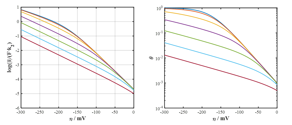
Figure 6.9. Scaled current density (left) and surface coverage (right) as a function of overpotential according to the Volmer-Heyrovský mechanism. K1 = 0.1 and k2/k−1 = 10−3, 10−2, 0.1, 1, 10 and 100 from top to bottom, pH = 2. Increasing K1 shifts the point where Tafel slope changes from 40 mV to 120 mV towards lower cathodic overpotentials (to the right).
6.5.2.2 Volmer-Tafel mechanism:
The analysis of the Volmer reactions remains the same, and the rate of the Tafel reaction can analogously be written as:
| 2 H* \(\ce{ ->[\ce{\nu_3}] }\) H2(g) | |
| \( \nu_3=-\frac{1}{2}\frac{d\theta}{dt}=k_3\theta^2 \) |
(6.83) |
|---|
The steady-state approximation is now d\( \theta \)/dt = v1 - v-1 - 2v3 = 0:
| \( k_1[\text{H}^+](1-\theta)e^{(\alpha-1)f\eta}-k_{-1}\theta e^{\alpha f \eta}-2k_3\theta^2=0 \) |
(6.84) |
|---|
Solving for the surface coverage \( \theta \) would require the solution of the second order algebraic equation, which would not be very demonstrative. We therefore look again at the limiting cases \( \theta \approx0 \) and \( \theta \approx1 \).
If \( \theta \approx0 \), the second order term of Equation (6.84) vanishes, and from the remaining equation
| \( \displaystyle\theta \approx \frac{k_1[\text{H}^+]}{k_1[\text{H}^+]+k_{-1}e^{f\eta}} \) |
(6.85) |
|---|
In order to have the surface coverage close to zero, it must be valid that k-1 » k1. Thus,
| \( \displaystyle\theta \approx\frac{k_1[\text{H}^+]}{k_{-1}} e^{-f\eta}=K_1[\text{H}^+]e^{-f\eta} \) | (6.86) |
|---|
| \( \displaystyle\frac{i}{F}=2k_3K_1^2[\text{H}^+]^2e^{-2f\eta} \) | (6.87) |
|---|
Equation (6.87) shows that the reaction is of the second order with respect to the proton concentration (see Eq. (6.79)). The Tafel slope is now
| \( \displaystyle\frac{\partial\eta}{\partial\text{ log }i}=2.303\frac{RT}{F} \approx30\text{ mV} \) | (6.88) |
|---|
If the surface coverage \( \theta \) approaches unity, it is obtained directly from Equation (6.84) that
| \( \displaystyle\frac{i}{F}=k_3=\text{constant} \) | (6.89) |
|---|
This condition is fulfilled if k1 » k-1, k3. The current would in this case be kinetically limited and not dependent on overpotential or pH.
A full simulation to Equations (6.83) and (6.84) is shown in Figure 6.10.
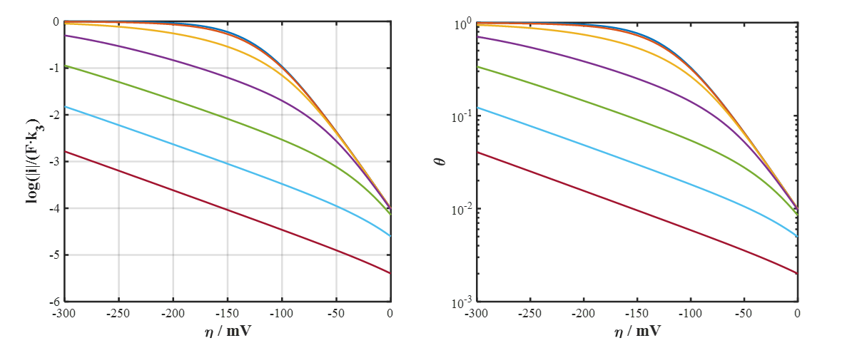
Figure 6.10. Scaled current density (left) and surface coverage (right) as a function of overpotential according to the Volmer-Tafel mechanism. K1 = 1 and k3/k−1 = 10−3, 10−2, 0.1, 1, 10 and 100 from top to bottom, pH = 2. Increasing K1 shifts the point where Tafel slope changes from 30 mV to infinity towards lower cathodic overpotentials (to the right).
6.5.2.3 Equilibrium and the rate-determining step
If the second step, be it of the Heyrovský or Tafel reaction, is rate-determining, the first step remains at equilibrium at all times. Writing this in calculus, v1 = v-1, and using Equation (6.72), an electrochemical Langmuir isotherm is obtained:
| \( \displaystyle\frac{\theta}{1-\theta}=K_1[\text{H}^+]e^{-f\eta} \Leftrightarrow \theta=\frac{K_1[\text{H}^+]e^{-f\eta}}{1+K_1[\text{H}^+]e^{-f\eta}} \) | (6.90) |
|---|
The rate of the net reaction depends on the prevailing mechanism (Heyrovský or Tafel). It is easy to show that the steady-state approximation used above, d\( \theta \)/dt = 0, is valid only when the second step is rate-determining. At high cathodic overpotentials, the surface coverage approaches unity, and at low overpotentials it approaches zero.
* S. Krzewska, Electrochim. Acta, 42 (1997) 3531. (acidic solution)
† \( K_1=\text{exp}[-f(E-E_1^{0'})] \)
‡ Tavakkoli et al. Angewandte Chemie, 54 (2015) 4535-4538.