CHEM-E4185 - Electrochemical Kinetics, 25.02.2019-29.05.2019

Impedance is a complex quantity, so one numerical value is not enough to describe it. There are many ways to represent impedance data [1], but the most common ones are Bode and Nyquist plots. A Bode plot, which is most commonly used in control systems and electrical engineering, shows the magnitude of impedance and the phase angle as a function of logarithm of frequency. The magnitude is commonly expressed in decibels, i.e. 20\( \times \)log|Z|. The phase angle has little relevance in control systems and electrical engineering.

Electrochemists prefer the a Nyquist plot or impedance plot, in which the real part of impedance Z’ is on the horizontal axis and the opposite number of the imaginary part -Z” is on the vertical axis at each frequency. This is because the imaginary part is usually negative. Frequency is not displayed explicitly in the Nyquist plot.

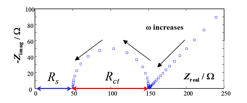
Figure 8.9. Nyquist (impedance) plot of Randles circuit.

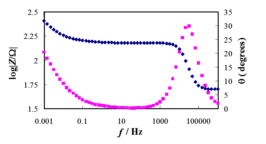
Figure 8.10. Bode plot of Randles circuit. Blue is the magnitude and pink is the phase angle.

The Nyquist and Bode plots of Randles circuit, one of the essential equivalent circuits describing electrochemical systems, is shown in Figures 8.9 and 8.10. For the authors of this book at least, the former is more informative because the ohmic resistance and charge transfer resistance, in other words the rate of charge transfer process, can be seen immediately. Bode plots are monotonically decreasing curves, in which the information is hidden in the negative slope and the points of inflection where the slope changes. In control systems engineering, the so called poles are of great interest, and this information can be obtained from the point of inflection. In this book, we will use almost exclusively Nyquist plots because of their clarity. Sometimes, however, it is more beneficial to show an admittance plot where the real part of admittance is on the horizontal axis and the imaginary part on the vertical axis.