CHEM-E4185 - Electrochemical Kinetics, 25.02.2019-29.05.2019
This course space end date is set to 29.05.2019 Search Courses: CHEM-E4185
Kirja
8. Impedance technique
8.5. Other diffusion elements
The Warburg element is a result of a semi-infinite
diffusion field, in which the boundary condition is a finite concentration at
an infinite distance from the electrode surface. Usually, however, instead of
this boundary condition, the concentration is defined at the distance \( \delta \), which can be, e.g. the thickness of a
membrane or an unstirred layer (see Section 7.2) Applying the boundary condition\( c_{\text{R}}(\delta)=c_{\text{R},0} \), the surface
concentration in the Laplace domain becomes
| \( \displaystyle\overline{c}_{\text{R}}^s=\frac{c_{\text{R,0}}}{s}-\frac{\overline{i}(s)}{nF\sqrt{D_{\text{R}}}}\frac{\tanh\left(\delta\sqrt{s/D_{\text{R}}}\right)}{\sqrt{s}} \) | (8.58) |
|---|
For the species ’O’, the expression becomes
respectively
| \( \displaystyle\overline{c}_{\text{O}}^s=\frac{c_{\text{O,0}}}{s}+\frac{\overline{i}(s)}{nF\sqrt{D_{\text{O}}}}\frac{\tanh\left(\delta\sqrt{s/D_{\text{O}}}\right)}{\sqrt{s}} \) | (8.59) |
|---|
Instead of the Warburg element, the diffusion impedance consists of two tanh elements.
If there is an insulating layer through which current does not flow at the distance \( \delta \), one must use the boundary condition| \(\displaystyle\left(\frac{\partial c_k}{\partial x}\right)_{x=\delta}=0 \) ; k = R,O |
(8.60) |
|---|
In this case, a hyperbolic tangent is replaced
by a hyperbolic cotangent:
| \( \displaystyle\overline{c}_k^s=\frac{c_{k,0}}{s}\mp\frac{\overline{i}(s)}{nF\sqrt{D_k}}\frac{\coth\left(\delta\sqrt{s/D_k}\right)}{\sqrt{s}} \) ; k = R,O | (8.61) |
|---|
The minus sign is for the species ’R’ and the
plus sign for the species ’O’. Impedance plots of various diffusion elements
have been compared in Figure 8.16, and it becomes evident that there are
differences only at very low frequencies
f < 1 Hz. From this, we obtain a diagnostic criterion, when the
thickness of the finite diffusion layer needs to be taken into account:
| \( \displaystyle\frac{\delta}{\sqrt{D}}\sqrt{f}<1 \) | (8.62) |
|---|
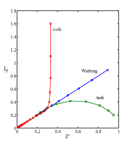
Figure 8.16. Diffusion elements tanh and coth compared to Warburg element. f = 0,1 ... 1000 Hz, \( \delta \)/√D = 1.
A typical value for the diffusion coefficient in water solution is 10-5 cm2s-1. If the lowest measurement frequency is 1 Hz, the diffusion layer has to be thinner than ca. 30 \( \mu \)m in order to observe differences compared to the Warburg element. If f = 0.1 Hz, the observed d increases to 100 \( \mu \)m. In practice, the use of tanh and coth elements is not common. At the boundary \( \delta\sqrt{f/D} \rightarrow0 \), a tanh element reduces to a resistor and coth element to a capacitor.
In the symmetrical thin layer cell in Figure 8.17, the following boundary condition holds:| \(\displaystyle \left(\frac{\partial c_k}{\partial x}\right)_{x=0}= \left(\frac{\partial c_k}{\partial x}\right)_{x=\delta} \) | (8.63) |
|---|
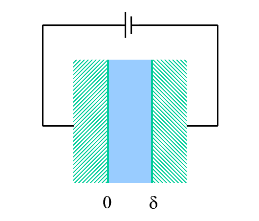
Thus the diffusion impedance is expressed as
| \( \displaystyle Z_{\text{diff}}=\frac{RT}{n^2F^2Ac_{k,0}}\frac{\tanh\left(\frac{1}{2}\delta\sqrt{j\omega/D_k}\right)}{\sqrt{j\omega}} \) | (8.64) |
|---|
Electrodes
with micrometer-sized dimensions are called (ultra) microelectrodes. The
diffusion field around these electrodes is almost spherical as shown in Figure 8.18.
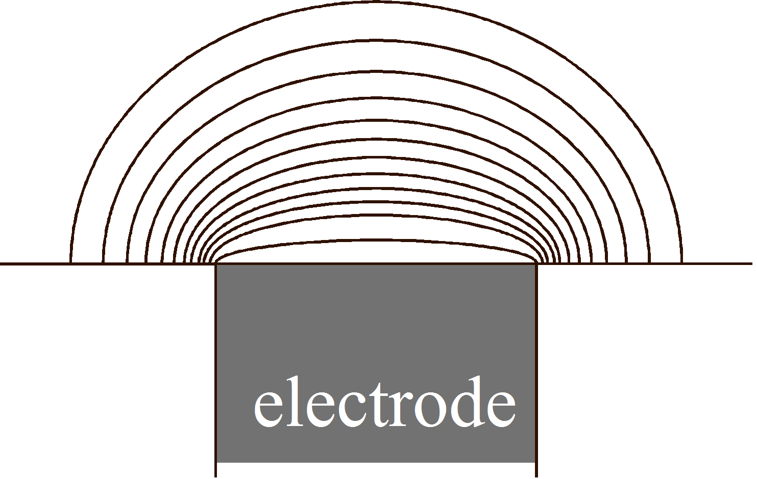
To be exact, the diffusion equation should be solved in cylindrical
coordinates, but in this case, the solution would contain modified Bessel
functions, which are not very illustrative.[1] We are satisfied with an approximation and use spherical coordinates. Now
Fick’s 2nd law becomes
| \( \displaystyle\frac{\partial c_k}{\partial t}=D_k\left[\frac{\partial^2c_k}{\partial r^2}+\frac{2}{r}\frac{\partial c_k}{\partial r}\right] \) | (8.65) |
|---|
The solution for the equation in the semi-infine diffusion field is
| \( \displaystyle\overline{c}_k=\frac{c_k^b}{s}+\frac{A(s)}{r}e^{-\lambda_kr} \) ; \( \displaystyle\lambda_k=\sqrt{\frac{s}{D_k}} \) |
(8.66) |
|---|
The current boundary condition for the species’R’ is expressed as
| \( \displaystyle D_{\text{R}}\left(\frac{\partial\overline{c}_{\text{R}}}{\partial r}\right)_{r=a}=\frac{\overline{i}(s)}{nF}=-\sqrt{D_{\text{R}}}\frac{A(s)}{a}e^{-\lambda_{\text{R}}a}\left(\sqrt{s}+\frac{\sqrt{D_{\text{R}}}}{a}\right) \) | (8.67) |
|---|
where a
is the radius of an electrode. The concentration on a sphere with a radius a is
| \( \displaystyle\overline{c}_{\text{R}}^s=\frac{c_{\text{R},0}}{s}-\frac{\overline{i}(s)}{nF\sqrt{D_{\text{R}}}}\frac{1}{\sqrt{s}+\sqrt{D_{\text{R}}}/a} \) | (8.68) |
|---|
Thus the diffusion impedance is
| \(\displaystyle Z_{\text{diff,}k}=\frac{RT}{n^2F^2Ac_{k,0}\sqrt{D_k}}\frac{1}{\sqrt{j\omega}+b} \) ; \( b=\frac{\sqrt{D_k}}{a} \) |
(8.69) |
|---|
The form \( (\sqrt{j\omega}+b)^{-1} \) corresponds to the parallel combination of Warburg element and a resistor (Figure 8.19). The graph of impedance is an arc of a circle \( Z'^2+Z''^2=Z'-Z'' \).
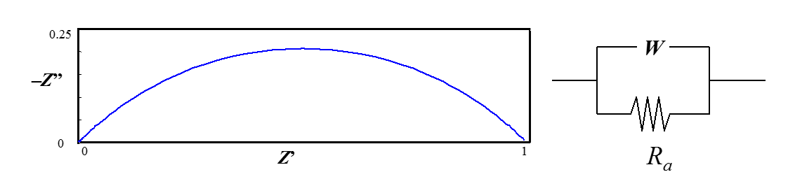
Figure 8.19. Diffusion impedance in spherical symmetry, b = 1.
If
the electrode reaction is coupled with a homogenous reaction, e.g. according to
the EC mechanism:
R – ne– \(\ce{ <=>[\ce{k(f)}][\ce{k(b)}] }\) O \(\ce{ ->[\ce{k(H)}] }\) products
where kH is the rate constant of a homogenous reaction, the solution for the species ’R’ is as before, i.e. Equation (7.7), but the diffusion equation of species ‘O’ becomes
| \( \displaystyle\frac{\partial c_{\text{O}}}{\partial t}=D_{\text{O}}\frac{\partial^2 c_{\text{O}}}{\partial x^2}-k_{\text{H}}c_{\text{O}} \) | (8.70) |
|---|
After taking the Laplace transform, the
solution is
| \( \displaystyle\overline{c}_{\text{O}}^s=\frac{c_{\text{O},0}}{s+k_{\text{H}}}+\frac{\overline{i}(s)}{nF\sqrt{D_{\text{O}}}}\frac{1}{\sqrt{s+k_{\text{H}}}} \) | (8.71) |
|---|
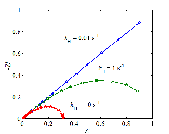
Thus it is evedent that the diffusion impedance of the species ’O’ is expressed as \( (j\omega+k_{\text{H}})^{-1/2} \), which is called the Gerischer impedance. The Gerisher impedance simulated with three different values of rate constants of a homogenous reaction are shown in Figure 8.20. Unlike in cyclic voltammetry, where small values of kH are more easily determined, the impedance technique tends to give higher values of kH. The impedance curve intersects the real axis at \( k_{\text{H}}^{-1/2} \). With small values of the rate constant of a homogenous reaction, the Gerischer impedance is identical to the Warburg impedance. Note that the shape of the Gerischer impedance resembles that of the tanh element presented in the previous section, which was a result of diffusion in a restricted space. If there is variation in the measurement data, it is crucial to know beforehand which processes are taking place in the system because otherwise a seemingly good fit into the equivalent circuit gives a misleading result. In practice, just like in the case of tanh and coth elements, the use of the Gerischer impedance is not common.
[1] The exact solution by Fleischmann and Pons can be found in J. Electroanal. Chem. 250 (1988) 277-283.