CHEM-E4185 - Electrochemical Kinetics, 25.02.2019-29.05.2019
This course space end date is set to 29.05.2019 Search Courses: CHEM-E4185
Kirja
8. Impedance technique
8.6. Corrosion
Impedance spectroscopy is also a good method for corrosion research. The typical corrosion reactions in acidic and basic
solutions are described in Section 6.5.4. Dissolution of a metal can formally
be written according to the Tafel equation:
| \(\displaystyle i_{\text{corr}}=i_{0,a}\left[e^{\alpha_anf(E_{\text{corr}}-E_a^0)}-e^{-\beta_anf(E_{\text{corr}}-E_a^0)}\right] \) |
(8.72) |
|---|
where i0,a is the exchange current density of the anode reaction, \( \alpha \)a and \( \beta \)a charge transfer coefficients, Ea0 equilibrium potential, and Ecorr corrosion potential of an electrode. If the cathode reaction is for example, hydrogen evolution, it can be considered irreversible, and
| \(\displaystyle i_{\text{corr}}=i_{0,c}e^{-\beta_cnf(E_{\text{corr}}-E_c^0)} \) |
(8.73) |
|---|
The quantities in Equation (8.73) correspond to those in Equation (8.72). The corrosion potential settles itself between the equilibrium potentials: \( E_c^0 < E_{\text{corr}} < E_a^0 \). If all variables in these equations are known based on, for example Tafel slopes, the corrosion potential can be solved because the anode and cathode reaction cancel each other out. If the equilibrium potentials are sufficiently far from one another, the inverse anodic reaction can be neglected and we have an expression derived by Stern and Geary for zinc dissolution with simultaneous hydrogen evolution [1]:
| \(\displaystyle i_{\text{corr}}=i_{0,a}e^{\alpha_anf(E_{\text{corr}}-E_a^0)}=i_{0,c}e^{-\beta_anf(E_{\text{corr}}-E_c^0)} \) | (8.74) |
|---|
Interpreting icorr as an exchange current of the corrosion reaction, the current-overpotential equation becomes
| \(\displaystyle i=i_{\text{corr}}(e^{\alpha_anf\eta}-e^{-\beta_cnf\eta}) \) | (8.75) |
|---|
where \( \eta \) = E - Ecorr. Hence the expressions for the currents can be linearized in the vicinity of \( \eta \) = 0:
| \( \displaystyle\frac{i}{i_{\text{corr}}}=1+\alpha_anf\eta-1+\beta_cnf\eta=(\alpha_a+\beta_c)nf\eta \Rightarrow \frac{i}{i_{\text{corr}}}=(\alpha_a+\beta_c)\frac{nF}{RT}R_p \) | (8.76) |
|---|
where Rp is polarization resistance. Corrosion current is easy to determine using the value of Rp, which is obtained from the diameter of the semicircle in the impedance plot. Often in corrosion literature the charge transfer coefficients are expressed in term of Tafel slopes (see Section 6.2.2), but more importantly, \( \alpha \)a + \( \beta \)c ≠ 1.
Corrosion
can be studied by setting the electrode at such a high anodic potential that
metal begins to dissolve. Then current naturally flows across the electrode and
the analysis becomes more complicated. Consider a two step mechanism, where
metal first forms a univalent cation M+, which remains adsorbed at
the surface. In the second step, the univalent cation is oxidized to a soluble
bivalent cation M2+.
| M \(\ce{ -> }\) M+* + e– | \( k_1=k_1^0e^{b_1\eta} \) |
|---|---|
| M+* \(\ce{ -> }\) M2+(aq) + e– | \( k_2=k_2^0e^{b_1\eta} \) |
k1 and k2 are the reaction rate constants of the steps and b1,2 = \( \beta \)1,2×F/RT.
Again, let the symbol \( \varphi \) denote the surface coverage of the adsorbed cation. Current is the sum of the first and second steps:
| \( \displaystyle\frac{i}{F\Gamma_{\text{max}}} =k_1(1-\varphi)+k_2\varphi \) | (8.77) |
|---|
The term k1(1 - \( \varphi \)) describes the process in which the metal is
only dissolved from the free surface. The mass balance for the adsorbed species
M+* is
| \( \displaystyle\frac{d\varphi}{dt} =k_1(1-\varphi)+k_2\varphi \) | (8.78) |
|---|
Surface coverage thus changes only due to
electrochemical reactions. In a steady state, d\( \varphi \)/dt = 0, and \( \varphi \)ss =k1/(k1 + k2).
After linearization and taking the Laplace transform of Equation (8.77):
| \( \displaystyle\frac{\Delta\overline{i}}{F\Gamma_{\text{max}}}=(1-\varphi_{ss})\Delta\overline{k}_1(s)-k_1\Delta\overline{\varphi}(s)+\varphi_{ss}\Delta\overline{k}_2(s)+k_2\Delta\overline{\varphi}(s)=[(1-\varphi_{ss})b_1k_1+\varphi_{ss}b_2k_2]\Delta\overline{\eta}(s)-(k_1-k_2)\Delta\overline{\varphi}(s) \) | (8.79) |
|---|
Using the expression for \( \varphi \)ss and after some algebra, we obtain
| \( \displaystyle \frac{\Delta\overline{i}(s)}{F\Gamma_{\text{max}}\Delta\overline{\eta}(s)}=\frac{(b_1+b_2)k_1k_2}{k_1+k_2}-(k_1-k_2)\frac{\Delta\overline{\varphi}(s)}{\Delta\overline{\eta}(s)} \) | (8.80) |
|---|
After linearization and taking the Laplace transform of Equation (8.76):
| \(\displaystyle s\Delta\overline{\varphi}(s)=(1-\varphi_{ss})\Delta\overline{k}_1(s)-k_1\Delta\overline{\varphi}(s)-\varphi_{ss}\Delta\overline{k}_2(s)-k_2\Delta\overline{\varphi}(s)=[(1-\varphi_{ss})b_1k_1-\varphi_{ss}b_2k_2]\Delta\overline{\eta}(s)-(k_1+k_2)\Delta\overline{\varphi}(s) \) |
(8.81) |
| \(\displaystyle \Rightarrow (s+k_1+k_2)\frac{\Delta\overline{\varphi}(s)}{\Delta\overline{\eta}(s)} =\frac{(b_1-b_2)k_1k_2}{k_1+k_2} \) | (8.82) |
|---|
Combining Equations (8.80) and (8.82) the
corrosion impedance is
| \( \displaystyle Z_{\text{corr}}^{-1}=FA\Gamma_{\text{max}}\frac{k_1k_2}{k_1+k_2}\left[b_1+b_2-\frac{(b_1+b_2)(k_1-k_2)}{k_1+k_2+j\omega}\right] \) | (8.83) |
|---|
The brackets include two terms, which means parallel elements because we are
dealing with admittance. The first term is independent of the frequency: hence it is a resistor. The reciprocal of the second term, i.e. its impedance form is, a sum of a frequency-independent term and another term that is directly
proportional to jω. This sum is therefore a series combination of a resistor
and an inductor. The total impedance is therefore
| \( \displaystyle Z_{\text{corr}}^{-1}=\frac{1}{R_t}+\frac{1}{R_{ad}+j\omega L_{ad}} \) | (8.84) |
|---|
The equivalent circuit and the capacitance of
the electrode as well as a simulated impedance plot are shown in Figure 8.21. The
expressions for the elements can be written as
| \( \displaystyle R_t=\frac{1/k_1+1/k_2}{FA\Gamma_{\text{max}}(b_1+b_2)} \) |
(8.85) |
|---|---|
| \(\displaystyle R_{ad}=-\frac{(1/k_1+1/k_2)(k_1+k_2)}{FA\Gamma_{\text{max}}(b_1-b_2)(k_1-k_2)} \) |
(8.86) |
| \(\displaystyle L_{ad}=-\frac{(1/k_1+1/k_2)\Gamma_{\text{max}}}{FA\Gamma_{\text{max}}(b_1-b_2)(k_1-k_2)} \) |
(8.87) |
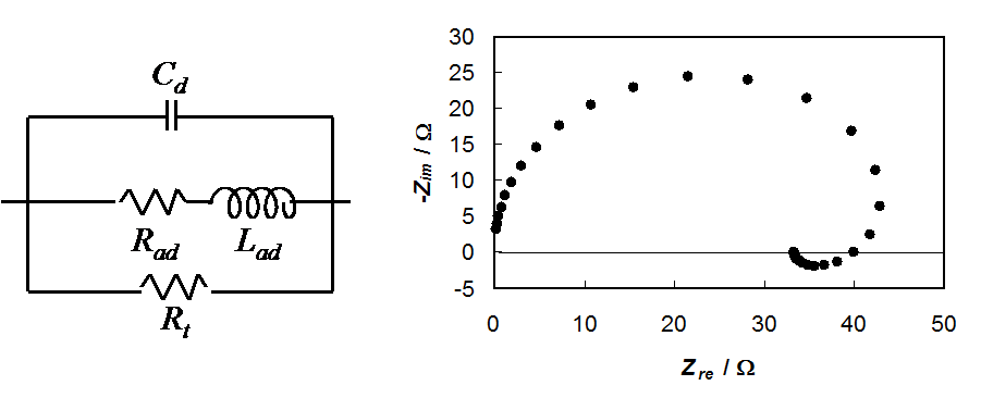
Figure 8.21. Equivalent circuit of corrosion impedance and a simulated impedance plot, Rt = 50 W, Rad = 100 \( \omega \), Lad = 0,01 H and Cd = 0,5 \( \mu \)F.
It is remarkable that Rad and Lad can have negative values, but they must have the same sign because
| \(\displaystyle \frac{L_{ad}}{R_{ad}}=\frac{1}{k_1+k_2} \) | (8.88) |
|---|
Reaction rate constants k1 and k2 can be determined from the values of the elements as follows:
| \( \displaystyle k_1=\frac{R_{ad}}{2L_{ad}}\left(1-\frac{b_1+b_2}{b_1-b_2}\frac{R_t}{R_{ad}}\right) \) |
(8.89) |
| \(\displaystyle k_2=\frac{R_{ad}}{2L_{ad}}\left(1+\frac{b_1+b_2}{b_1-b_2}\frac{R_t}{R_{ad}}\right) \) | (8.90) |
|---|
The factors b1 and b2 must be determined separately, e.g. from Tafel slopes. If they are equal, the impedance is simplified to Rt (see Equation (9.92)).
The characteristic feature of corrosion impedance is the inductive loop below the real axis at low frequencies. If there are several adsorption steps, each of them will give its own loop. At high frequencies, an inductive loop below the real axis is sometimes seen, but it is due to the wires connecting the cell and the measurement apparatus (potentiostat). It can be modeled as an inductor in series with the solution resistance.