CHEM-E4185 - Electrochemical Kinetics, 25.02.2019-29.05.2019
This course space end date is set to 29.05.2019 Search Courses: CHEM-E4185
Kirja
8. Impedance technique
8.8. Transmission lines
A transmission line is an alternative way to
describe charge transfer mechanisms. A schematic representation of a
transmission line is shown in Figure 8.25.

Figure 8.25. Simple transmission line.
The same transmission line can be drawn in an
electrically identical form, which enables the determination of the impedance
of the whole transmission line.
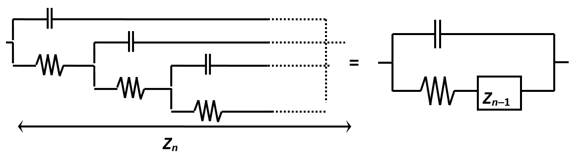
From the right-hand side of the scheme of Figure 8.26, the impedance can
be determined as follows:
| \( \displaystyle Z_n=\frac{1}{j\omega C+\frac{1}{R+Z_{n-1}}} \) | (8.95) |
|---|
Because of the infinite length of the transmission line, Zn = Zn-1 = Z, and Z can be solved:
| \( \displaystyle Z=\frac{R}{2}\left(\sqrt{1+\frac{4}{j\omega RC}-1}\right) \approx\sqrt{\frac{R}{j\omega C}} \) | (8.96) |
|---|
Equation (8.96) is of the form (j\( \omega \))-1/2, that is the Warburg impedance. The following is given without proof: If the length of the line is finite and the end of the line short-circuited, the line represents the tanh element. If the end of the line is open, it is the coth element, see Figure 8.16.
The
impedance plot of a porous membrane is a semicircle, which is a little difficult
to understand. If a pore in the membrane is modeled as a straight capillary
with a given surface charge density and filled with an electrolyte solution,
the following transmission line can be drawn, which originally describes an
electric conductor with finite conductivity:
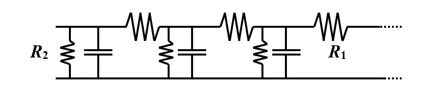
Figure 8.27. Transmission line of a conductor with a finite conductivity.
Analogously to Figure 8.26, this line can be redrawn as:
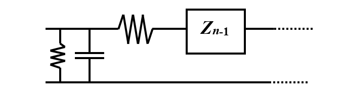
Figure 8.28. Reduced transmission line of Figure 8.27.
Again, the impedance can be solved assuming the
line infinite:
| \( \displaystyle\frac{1}{Z_n}=j\omega C+\frac{1}{R_2}+\frac{1}{R_1+Z_{n-1}} \Rightarrow Z=\frac{R_1}{2} \left(\sqrt{1+\frac{4}{R_1(1/R_2+j\omega C)}}-1\right) \) | (8.97) |
|---|
Taking into account that with small values of x,
\( \sqrt{1+x} \approx1+\frac{1}{2}x \) and
Equation (8.97) can be expressed as:
| \( \displaystyle Z \approx\frac{1}{1/R_2+j\omega C} \) | (8.98) |
|---|
This is the parallel combination of C and R2, which gives the desired semicircle [1].
[1] If you are wondering about the approximations or the conclusions drawn, it is easy to check the validity of them using any mathematical software (Matlab, Mapple, Mathematica) and realize that the impedance plots can be constructed even without approximations.