CHEM-E4185 - Electrochemical Kinetics, 25.02.2019-29.05.2019
This course space end date is set to 29.05.2019 Search Courses: CHEM-E4185
Kirja
3. Transport in electrolyte solutions
3.4. Analysis of transport equations in a steady state
The Nernst-Planck equation must be written out for each species in the solution. Constraints of the group of equations are the electroneutrality condition and electric current density:
| \( \displaystyle\sum\limits_{k}z_kc_k=0 \) | (2.3) |
|---|
| \(\displaystyle i=F\sum\limits_{k}z_kJ_k \) | (3.14) |
|---|
The solution of the group is possible in closed form,2 but let us highlight a couple of its important features with the help of a binary electrolyte \( A_{\upsilon_+}B_{\upsilon_-} \). Division by diffusion coefficients gives
| \( \begin{cases}-\displaystyle\frac{J_+}{D_+}=\nabla c_{+}+\displaystyle\frac{z_+F}{RT}c_+\nabla\phi-\displaystyle\frac{v}{D_+}c_+ \\ -\displaystyle\frac{J_-}{D_-}=\nabla c_{-}+\displaystyle\frac{z_-F}{RT}c_-\nabla\phi-\displaystyle\frac{v}{D_-}c_-\end{cases} \) | (3.38) |
|---|
Ionic concentrations are c+
= \( \upsilon \)+c and c- = \( \upsilon \)-c, and the condition of electroneutrality can be written as z+\( \upsilon \)+ + z-\( \upsilon \)- = 0. Summing above equations, \( \nabla\phi \) is eliminated:
| \( \displaystyle\frac{J_+}{D_+}-\frac{J_-}{D_-}=(\upsilon_++\upsilon_-)\nabla c-\left(\frac{\upsilon_+}{D_+}+\frac{\upsilon_-}{D_-}\right)vc \) | (3.39) |
|---|
With equation (3.14) and electroneutrality, the left had side of Equation (3.39) can be written as
| \(\displaystyle -J_+\left(\frac{1}{D_+}-\frac{z_+}{z_-D_-}\right)-\frac{i}{z_-D_-F}=-J_+\left(\frac{1}{D_+}+\frac{\upsilon_-}{\upsilon_+D_-}\right)-\frac{i}{z_-D_-F} \) |
(3.40) |
|---|
and equation (3.38) using straightforward algebra:
| \( \begin{cases}J_+=-\displaystyle\frac{(\upsilon_++\upsilon_-)D_+D_-}{\upsilon_-D_++\upsilon_+D_-}\nabla c_++\frac{D_+}{z_+D_+-z_-D_-}\displaystyle\frac{i}{F}+vc_+\\J_-=-\displaystyle\frac{(\upsilon_++\upsilon_-)D_+D_-}{\upsilon_-D_++\upsilon_+D_-}\nabla c_--\displaystyle\frac{D_-}{z_+D_+-z_-D_-}\displaystyle\frac{i}{F}+vc_-\end{cases} \) | (3.41) |
|---|
The coefficient of the concentration gradient is the electrolyte diffusion coefficient D±:
| \( \displaystyle D_{\pm}=\frac{(\upsilon_++\upsilon_-)D_+D_-}{\upsilon_-D_++\upsilon_+D_- } \Leftrightarrow \frac{\upsilon_++\upsilon_-}{D_{\pm}} =\frac{\upsilon_+}{D_+}+\frac{\upsilon_-}{D_-} \) |
(3.42) |
|---|
Equation (3.42) is known as the Nernst-Hartley equation. It is important to notice that, in principle, only components, viz electrolyte diffusion coefficients can be measured, although an electrochemical measurement with a supporting electrolyte gives a very accurate approximation of an ionic diffusion coefficient – this case known as a trace ion case is discussed later. It is easy to use Equation (3.41) to check that z+J+ + z-J- = i/F. The coefficient in front of \( (i/F) \) is \( (t_i/z_i) \) where ti is the transport number of the ion. It is a measurable quantity (see paragraph 3.4.1) that tells us how large a fraction of electric current the ion carries in the solution. Adding up the convective terms of either Equation (3.33) or (3.41) gives \( v\sum_iz_ic_i=0 \), which tells us something elser important: electric current does not depend on convection. [1]
The ratio of the electrolyte diffusion coefficient and the cation transport number gives:
| \( \displaystyle\frac{D_{\pm}}{t_+}=\frac{(\upsilon_++\upsilon_-)D_+D_-}{\upsilon_-\left(D_++\frac{\upsilon_+}{\upsilon_-}D_-\right)}\frac{z_+\left(D_++\frac{\upsilon_+}{\upsilon_-}D_-\right)}{z_+D_+}=\left(1+\frac{\upsilon_+}{\upsilon_-}\right)D_- \) | (3.43) |
|---|
that gives the desired connection between ionic diffusion coefficients and measurable quantities. Now we are able to write down the Nernst-Planck equation in a compact form of
| \( \displaystyle\begin{cases}J_+=-D_{\pm}\nabla c_{+}+\displaystyle\frac{t_+i}{z_+D_+}+vc_+\\J_-=-D_{\pm}\nabla c_{-}+\displaystyle\frac{t_+-}{z_-D_-}+vc_-\end{cases} \) | (3.44) |
|---|
Starting from the definition of the transport number, i.e. the fraction of carried current, the following alternative forms can be achieved using Equations (3.14) and (3.15):
| \(\displaystyle t_k=\frac{z_kJ_k}{\sum\limits_{m}z_mJ_m}=\frac{z_ku_kc_k}{mz_mu_mc_m}=\frac{z_k^2D_kc_k}{\sum\limits_mz_k^2D_mc_m}=\frac{\lambda_kc_k}{\sum\limits_m\lambda_mc_m} \) | (3.45) |
|---|
You can check using a 2:1 electrolyte \( (z_+=2, \upsilon_+=1, z_-=-1, \upsilon_-=2) \), or example, that Equations (3.44) and (3.41) give the same result.
Combining Equations (3.38) and (3.44), a very important result is achieved: [2]
| \( \displaystyle\nabla\phi=-\frac{RT}{F} \left[ \frac{D_+-D_-}{z_+D_+-z_-D_-}\nabla\text{ln}c_++\frac{i/F}{z_+c_+(z_+D_+-z_-D_-)}\right]=-\frac{RT}{F}\left(\frac{t_+}{z_+}+\frac{t_-}{z_-}\right)\nabla\text{ln}c_+-\frac{i}{\kappa} \) | (3.46) |
|---|
Equation (3.46) states that the potential gradient in the solution is formed from two contributions, diffusion potential and ohmic loss. Diffusion potential arises from the differences in the ionic mobility. Although, say, a cation has a higher mobility than an anion (see Equation (3.5)), they must move at the same velocity in order to retain electroneutrality. This means that the anion is slowing down the movement of the cation and, accordingly, the cation is speeding up the movement of the anion. This is seen as diffusion potential. The magnitude of diffusion potential is, however, rather small because the ionic mobilities are usually of the same order of magnitude (H+ and OH- are exceptions due to their different transport mechanism). Ohmic loss, in contrast, is always present in the measurements; it is irreversible in nature because it leaves a system as a heat loss (Joule heat). Check with a 2:1 electrolyte that Equation (3.46) truly gives the term \( 1/ \kappa \).
It is easy to show that Equation (3.46) can be written in the general form of
| \( \displaystyle\nabla\phi=-\frac{RT}{F}\sum\limits_k\frac{t_k}{z_k}\nabla\text{ln}c_k-\frac{i}{\kappa} \). | (3.47) |
|---|
In systems with more than two ions, the use of the above equation is hampered because transport numbers are no longer constants but instead depend on the local concentrations of ions. In electrochemical experiments, the problem is circumvented by adding an excess of a supporting electrolyte at least 50 times the amount of the electroactive ion that reacts on the electrode. This makes the transport number of the electroactive ion practically zero, it is transported solely by diffusion and the supporting electrolyte is primarily carried by current. An ion such as this is called a trace ion. On the electrode, however, the situation is completely reversed because the trace-ion carries all the current:
| \( \displaystyle J_k|_{\text{surface}}=\frac{i}{nF}=-D_k\nabla c_k|_{\text{surface}} \) | (3.48) |
|---|
If the trace-ion is not converted to another trace-ion via the reaction, n = |zk|. In the following chapters we will see how an electrochemical measurement results in an ionic diffusion coefficient. Strictly speaking, it does not provide an entirely correct value because the concentration difference in the trace ion between the bulk and the surface – as small as it is – forces a similar difference in the counter-ion of the supporting electrolyte. However, since the supporting electrolyte moves mostly via migration (transport number » 0) it is able to react rapidly to the trace ion movement, i.e. to adjust its concentration profile and compensate for the trace ion charge. The compensation occurs instantaneously, causing only a tiny disturbance in the trace ion: the fluxes of the trace-ion and the supporting ion are said to be weakly coupled. A more thorough analysis of ionic coupling would require a deeper look at the theory of irreversible thermodynamics that is beyond the scope of this book.
3.4.1 Measurement of transport number
The measurement of the transport number is one of the oldest electrochemical measurements. There are basically three methods: the Hittorf method, the method of a moving boundary and the electromotive force of a cell with transference. In the Hittorf method, cathode and anode compartments are connected via a thin capillary, with no concentration gradient allowed to be formed during the experiment. When a charge of \( Q=I\Delta t \) is run through the cell, Q/(z+F) mol of cations has been removed from the cathode compartment but the amount of cations that have arrived is only t+Q/(z+F) mol. Their difference thus is \( \frac{(t_+-1)Q}{z_+F} \). A similar analysis can be done for the anode compartment. The transport number can be calculated by analyzing the composition of the cathode and anode compartments after the experiment.
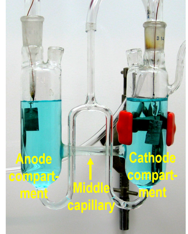
The disadvantage of the Hittorf method is that the duration of an experiment cannot be very long in order to prevent a concentration gradient from forming in the capillary connecting the compartments. During a brief experiment only rather small changes in concentrations occur, meaning the chemical analysis may be inaccurate. Current cannot be increased to an unlimited extent either because it would dissipate in the cell as heat.
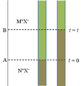
In the method of a moving boundary, a vertical capillary is equipped with a cathode on the top and an anode on the bottom. Two solutions with a common ion (M+X– and N+X–) are poured into the capillary, with the denser solution on the bottom. In order to keep the boundary between the solutions sharp, the mobility of M+ must be higher than that of N+. The boundary resides initially at position A (see Figure 3.7). The system is electrolyzed with the charge \( Q=I\Delta t \), causing M+ to move upwards towards the cathode. The amount of M+ transferred is (t+Q)/(z+F) mol; the boundary is now at a new position B. The amount of M+ removed from the interval A-B is \( c_{MX}A\Delta x \) (A is the area of the cross section of the capillary and \( \Delta x \) the distance A-B). Equating these two expressions we find that
| \( t_+=\displaystyle\frac{z_+c_{MX}\Delta xAF}{I\Delta t} \) | (3.49) |
|---|
The ingenuity of the method is that the boundary remains sharp and diffusion does not blur it. The lower and denser solution usually contains an indicator so the boundary can be observed with the naked eye.
The velocity of an ion is given by Equation (3.5): vi = uiE. Since the conductivity of the lower solution, κ, is lower than in the upper solution the electric field E ~ i/κ is stronger in the lower solution. If M+ diffuses into the lower solution the stronger electric field accelerates it back into the upper solution, separating it from N+ that has lower mobility than M+. Accordingly, if N+ diffuses into the upper solution it experiences a lower electric field that decelerates it and it lags behind M+, bringing it back to the lower solution. However, if the conductivity of the lower solution is higher than in the upper solution the boundary does not remain sharp. A more detailed explanation is given in, I.N. Levine Physical Chemistry, McGraw-Hill, Tokio 1978, page 458-9 (removed from later editions!). |
|---|
Perhaps the most elegant method of determining a transport number is based on the electromotive force of a cell with transference, that is, its open circuit potential. For example, if two NaCl solutions at different concentrations are separated by a porous membrane or a frit that allows ions to diffuse across, Equation (3.46) gives the following for the diffusion potential (i = 0):
| \( \displaystyle \Delta\phi=\pm\frac{(2t_+-1)RT}{F}\text{ln}\left(\frac{c^\alpha}{c^\beta}\right) \) | (3.50) |
|---|
where \( \alpha \) and \( \beta \) refer to the two compartments. If the electrodes are reversible to Cl– anions, the Nernst equation contributes to the open circuit potential, making the total potential
| \( \displaystyle E=\pm\frac{2t_+RT}{z_+F}\text{ln}\left(\frac{a_{\text{Cl}}^\alpha}{a_{\text{Cl}}^\beta}\right) \) | (3.51) |
|---|
where concentrations are replaced by activities (see Equation (3.36)). The sign must be chosen depending on which concentration \( (c^{ \alpha} \text{ or } c^{\beta}) \) is higher. The measurement must be carried out with a voltage meter that has a very high input impedance to keep the current zero. The concentration difference between the compartments cannot be very large either. Cell potentials are revisited in Chapter 4.