CHEM-E4185 - Electrochemical Kinetics, 25.02.2019-29.05.2019
This course space end date is set to 29.05.2019 Search Courses: CHEM-E4185
Kirja
7. Electrochemical methods
7.1. Transient methods
The analysis of all transient methods starts from Fick’s second law, Equation (3.54) and the boundary condition (3.48). We only consider a trace ion in a one-dimensional, semi-infinite space x ≥ 0. The Fick’s 2nd law is first converted into the Laplace domain:
| \( \displaystyle\frac{\partial c_i}{\partial t}=D_i \frac{\partial ^2c_i}{\partial x^2} \Rightarrow s\bar c-c_i^b=D_i\frac{d^2\bar c_i}{dx^2} \) | (7.1) |
|---|
where the upper bar denotes a variable in the Laplace domain; \( c_i^b \) is the initial or the bulk concentration of ion i, and s is the Laplace variable*. The general solution of this ordinary differential equation is
| \( \displaystyle\bar c_i(x,s)=\frac{c_i^b}{s}+A(s)e^{- \lambda_ix}+B(s)e^{- \lambda_ix}, \lambda_i=\sqrt{\frac{s}{D_i}} \) | (7.2) |
|---|
A(s) and B(s) are constants that are determined from the boundary conditions. In order to keep the concentration finite when x → ∞, B(s) must be zero. Boundary condition (3.48) gives:
| \( \displaystyle\frac{\bar i(s)}{nF}=-D_i\left(\frac {d \bar c_i}{dx}\right)_{x=0}=\sqrt{sD_i}A(s) \Rightarrow A(s)= \frac{\bar i(s)}{nF \sqrt{sD_i}} \) | (7.3) |
|---|
| \( \displaystyle\bar c_i(0,s)=\frac{c_i^b}{s}+ \frac{\bar i (s)}{nF\sqrt{sD_i}} \) | (7.4) |
|---|
Equation (7.4) is completely general as it was derived without assumptions related to any particular method. In order to proceed, we have to define the experimental method.
7.1.1 Potential step
In the potential step method, the electrode potential is stepped at t = 0 to a new value and then kept constant. If the reaction is reversible, the surface concentrations of the redox couple obey the Nernst equation:
| \( \displaystyle\left(\frac{c_{\text{o}}}{c_{\text{R}}}\right)_0=\text{exp}\left[\frac{nF}{RT}(E-E^{0'})\right]= \theta=\text{constant} \) | (7.5) |
|---|
| \( \displaystyle\Rightarrow \bar c_o(0,s)= \theta \bar c_R(0,s) \) | (7.6) |
|---|
Let us assume that we initially only have reduced species R present and the potential step is made in the anodic direction, i > 0, whereby cR at the electrode surface is lowered due to its oxidation. Hence
| \( \displaystyle\bar c_R(0,s)=\frac{c_{R,0}}{s}-\frac{\bar i(i)}{nF \sqrt{sD_o}} \) | (7.7) |
|---|
| \( \displaystyle\bar c_o(0,s)=\frac{\bar i(s)}{nF\sqrt{sD_o}} \) | (7.8) |
|---|
because \( c_o^b=0 \). Using Equation (7.6) current density \( \bar i_s \) can be solved:
| \( \displaystyle\bar i(s)= \frac{nF \sqrt {D_\text{o}}\theta c_{R}^b}{1+ \xi \theta } \frac{1}{\sqrt{s}}, \xi=\sqrt\frac{D_{\text{O}}}{D_{\text{R}}} \) | (7.9) |
|---|
Current density in the time domain is obtained by an inverse transformation that can be found in the Table of Laplace transforms (Appendix 5):
| \(\displaystyle \bar i(t)= \frac{nF \sqrt {D_\text{o}}\theta c_{R}^b}{1+ \xi \theta } \frac{1}{\sqrt{\pi t}} \) | (7.10) |
|---|
If the potential is stepped to such high anodic potential \( \xi \theta \gg1 \) that the surface concentration of R immediately drops to zero, we see directly from Equation (7.7) that
| \( \displaystyle\vec{i}_d(s)= \frac{nF \sqrt {D_\text{R}} c_{R}^b}{\sqrt{s}} \Rightarrow \vec{i}_d(t)= \frac{nF \sqrt {D_\text{R}} c_{R}^b}{\sqrt{\pi t}} \) | (7.11) |
|---|
Equation (7.11) is known as the Cottrell equation, which states that, along with Equation (7.10), current under diffusion control decays in a manner proportional to t−1/2. These equations bear the peculiarity that at time t = 0 current should be infinite. This naturally never happens because a small solution resistance Rs always remains between the electrode and the Luggin capillary (see Chapter 4). Current at t = 0 is therefore equal to \( \Delta E/R_s \) where \( \Delta E \) is the height of the potential step. Electrodes also always have double layer capacitance, Cdl, and charging this capacitance makes current decay exponentially, \( i_c=(\Delta E/R_s)e^{-t/(R_sC_{dl})} \) Total current is the sum of this charging current, ic, and diffusion current, Equation (7.10) or (7.11). Charging time is, however, very short on solid electrodes, only a few microseconds, and usually we do not notice it at all.
The current from Equation (7.10) can be written in terms of the Cottrell current, Equation (7.11):
| \(\displaystyle i(t)=i_d(t)\frac{ \xi \theta }{1+ \xi \theta } \) | (7.12) |
|---|
Solving for \( \xi \theta \) gives
| \(\displaystyle \xi \theta=\frac{i(t)}{i_d(t)-i(t)} \) | (7.13) |
|---|
Taking the logarithm and using the definition of \( \theta \), Equation (7.5), we end up with the result
| \( \displaystyle E=E^{0'}-\frac{RT}{nF}\text{ln} \xi- \text{ln} \frac{i_d(t)-i(t)}{i(t)} \) | (7.14) |
|---|
When current \( i(t)=\frac{1}{2}i_d(t) \), the final term of this equation vanishes and we have reached the half-wave potential E1/2:
| \( \displaystyle E_{1/2}=E^{0'}+\frac{RT}{nF}\text{ln}\sqrt{\frac{D_{\text{R}}}{D_{\text{O}}}} \) | (7.15) |
|---|
If instead of Equation (3.48) the boundary
condition ci (0,t) = 0 is used, which corresponds to the
Cottrell equation, the consentration profile can be calculated easily. In this case,
\( A(s)=-c_{i,0}/s \) and the concentration
in the Laplace domain is
Inverse transform is again found in the table of Laplace transforms:
Figure 7.1. Development of concentration profile during potential step experiment, Equation (7.17). D = 10-5 cm2/s. |
|---|
If an electrode reaction has a limited rate, the Nernst equation (7.5) cannot be used as the boundary condition, but Equation (6.12) is used instead. In the Laplace domain it reads
| \( \displaystyle\frac{\bar i(s)}{nF}=k_{ox}\bar c_{\text{R}}(0,s)-k_{red}\bar c_{\text{O}}(0,s) \) | (7.18) |
|---|
where kox and kred are the rate constants of the oxidation and reduction reactions, respectively, as discussed in the previous chapter. Inserting the surface concentrations, Equations (7.7) and (7.8), into this equation, current density takes on the following form:
| \(\displaystyle \frac{\bar i(s)}{nF}=\frac{k_{\text{ox}}c_{\text{R,0}}}{\sqrt{s}} \frac{1}{\sqrt{s}+k_{ox}/\sqrt{D_{\text R}}+k_{red}/\sqrt{D_{\text{o}}}} \) | (7.19) |
|---|
Equation (7.19) is of the form \( \frac{1}{\sqrt{s}(\sqrt{s}+\lambda)} \) for which the inverse transform is found tabulated:
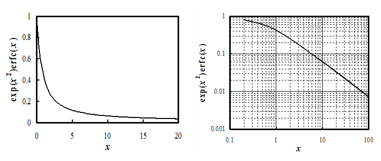
| \( \displaystyle\frac{i(t)}{nF}=k_{ox}c_{\text{R}}^b\text{exp}(\lambda^2t)\text{erfc}(\lambda\sqrt{t}) ; \lambda=\frac{k_{ox}}{\sqrt{D_{\text{R}}}}+\frac{k_{red}}{\sqrt{D_{\text{O}}}} \) | (7.20) |
|---|
When \( x=0, \text{exp}(x^2)\text{erfc}(x)=1 \),21F† making current density at t = 0 equal to \( i=nFk_{ox}c_{\text{R}}^b \). Since all reactions have a limited rate (value of the rate constant), the formal singularity in the Cotrell equation cannot exist in reality. The graph of Equation (7.20) approaches the time dependence t-1/2 at longer times, i.e. diffusion always steps in to limit the current (see Figure 7.2).
At low values of x the function can be linearized, and current density is given by:
| \( \displaystyle\frac{i(t)}{nF}=k_{ox}c_{\text{R}}^b\left(1-\frac{2\lambda\sqrt{t}}{\sqrt{\pi}}\right) \) | (7.21) |
|---|
Plotting current density as a function of \( \sqrt{t} \) and extrapolating to zero, the intercept at the current axis gives the value of kox. In principle, this could be seen directly from current at t = 0, but this value may be blurred due to the charging current or the limited response time of the potentiostat.
Potential steps are mainly used to determine electrochemical rate constants, as indicated above. In systems in which an electrode reaction is accompanied by a homogeneous reaction, a second step to the reverse potential can be made. The response to the second step now depends on the rate of the homogeneous reactions, which can be utilized in the analysis; these problems are beyond the scope of this book.
7.1.2 Linear potential scan or cyclic voltammetry
Linear potential scan or cyclic voltammetry is probably the most commonly applied electrochemical method. Although its calculus is more complicated than that of a potential step above, and although the accurate determination of kinetic parameters is prone to errors from various sources, it is an excellent semi-quantitative method. With reasonable training and experience, it is easy to deduce what kind of phenomena will prevail in the system. Estimates of the electrode reaction rate and the number of electrons exchanged are readily available, and the presence of an adsorption step or a following homogeneous reaction can easily be detected, for example. More specific reaction mechanisms, such as disproportionation also have their own very characteristic responses. The analysis of an electrochemical system is therefore commonly initiated with potential scans at varying scan rates, after which a more specific method can be chosen that applies to that particular problem.
As the name tells, the
electrode potential is scanned linearly as a function of time. If the scan is
reversed immediately from the end value back to the initial potential, the
procedure is called cyclic voltammetry. The scan rate is usually kept the same
in the forward and backward scans, although this is not mandatory; the theory of
cyclic voltammetry has been developed for constant scan rates. The potential
function in cyclic voltammetry can formally be written as
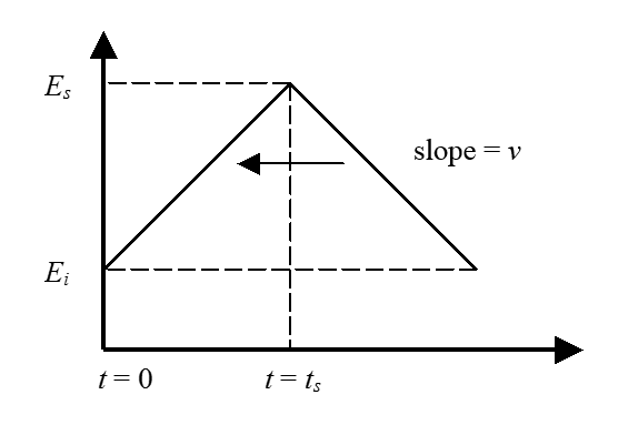
| \( \displaystyle E=E_i+vt-2H(t-t_s) v(t-t_s) \) | (7.22) |
|---|
where Ei is the initial potential, v the scan rate (\( Vs^{-1} \)), and ts the time of the scan reversal; the corresponding potential is accordingly Es (’s’ = switching). The scan rate v can be either positive or negative. \( H(t-t_s) \) is the Heaviside step function that has the value zero when t < ts and unity when \( t \geq t_s \).
Because the quantity \( \theta \) in Equation (7.5) is no more constant, the
Nernst equation cannot be transformed to the Laplace domain (Equation (7.6)). Instead,
the boundary condition is written as
| \( \displaystyle\frac{c_{\text{O}}(0,t)}{c_{\text{R}}(0,t)}= \theta_ie^{ \sigma t-2H(t-t_s) \sigma(t-t_s)}= \theta_iS(t) \) | (7.23) |
|---|
where \( \theta _i=\text{exp}[\frac{nF}{RT}(E_i-E^{0'})]] \) and \( \sigma=\frac{nF}{RT} v \) ; \( \sigma \) has the dimension s−1. The surface concentrations, Equation (7.4), are transformed back to the time domain using the convolution theorem:
| \( \displaystyle c_{\text{R}}(0,t)=c_{\text{R}}^b-\frac{1}{nF \sqrt{\pi D_{\text{R}}}} \int_{0}^{t}{\frac{i(u)du}{\sqrt{t-u}}} \) | (7.24) |
|---|
| \( \displaystyle c_{\text{O}}(0,t)=c_{\text{O}}^b-\frac{1}{nF \sqrt{\pi D_{\text{O}}}} \int_{0}^{t}{\frac{i(u)du}{\sqrt{t-u}}} \) | (7.25) |
|---|
In the above
equations, u is the dummy time
variable. Inserting Equations (7.24) and (7.25) into Equation (7.23) we find that
| \( \displaystyle\int_{0}^{t}{\frac{i(u)du}{\sqrt{t-u}}}=\frac{nF \sqrt{\pi D_{\text{O}}}}{1+ \xi \theta_iS(t)} \) | (7.26) |
|---|
\( \xi \) is defined earlier. The problem is reduced to the solution of the convolution integral on the left-hand side where the current function resides. In addition, the integral has a singularity at the upper integration limit. Equation (7.26) is written in a dimensionless form for the numeric solution. The time variable u is replaced with a dimensionless potential variable \( \theta= \sigma u \), leading to \( du=d \tau/ \sigma \). The current function i(u) is formally replaced with a new function \( g( \tau) \). The convolution integral is now in the form of
| \( \displaystyle\int_{0}^{t}{\frac{i(u)du}{\sqrt{t-u}}}=\frac{1}{\sqrt{\sigma}} \int_{0}^{\sigma t}{\frac{g(\tau)d \tau}{\sqrt{\sigma t-\tau}}} \) | (7.27) |
|---|
This is further divided by \( nF\sqrt{\pi D_{\text{O}}}c_{\text{O}}^b \), resulting in the dimensionless current function \( \chi( \tau) \):
| \(\displaystyle \int_{0}^{\sigma t}{ \frac{\chi(\tau)d\tau}{\sqrt{\sigma t-\tau}}}=\frac{\theta_iS(t)C_r-1}{1+ \xi \theta_iS(t) }; \chi(\tau)=\frac{g(\tau)}{cFc_{\text{O}}^b \sqrt{\pi D_{\text{O}}\sigma}} \) | (7.28) |
|---|
where \( C_r=c_{\text{O}}^b/c_{\text{R}}^b \). The real physical current (density) is expressed by the dimensionless current (density) as
| \(\displaystyle i(t)=g(\sigma t)=nFc_{\text{O}}^b\sqrt{\pi D_{\text{O}}\sigma}\chi(\sigma t) \) | (7.29) |
|---|
If only species ‘R’ is initially present,\( c_{\text{R}}^b \) is replaced with \( c_{\text{O}}^b \), Cr = 1, and unity vanishes from the numerator of the right hand side of Equation (7.28).
Integral equation (7.28) must be solved numerically. The best known methods is that of Nicholson and Shain in 1964 [1]. Integration by parts removes the singularity at the upper limit:
The
first term on the right-hand side vanishes at the upper limit, and because the
experiments are initiated at the potential where current is zero, it also vanishes at the lower limit. The second term is replaced with a sum, dividing \( \sigma \)t to
subintervals: \( \sigma t=N\delta \) and \( \tau=k\delta \) where
k = 0, 1, 2, ... , N.
Equation (7.31) thus assumes that in the interval [k, k+1] the term \( \sqrt{N-k} \) is nearly constant and can be moved in front of the integral sign, and from here \( d\chi \) can be integrated. Summing is easily done with a computer script. Current is calculated using the values calculated previously:
|
|---|
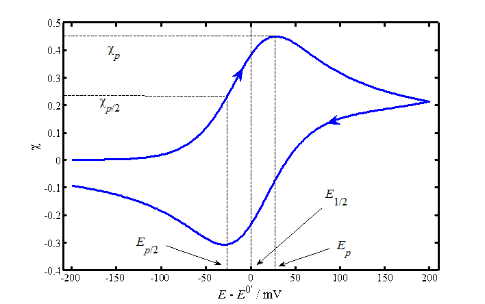
The numeric solution of the convolution integral gives the following diagnostic criteria for a reversible reaction:
1. The peak current density, ip, is
\( \displaystyle i_p=0.4463nFc_{O}^b\sqrt{\frac{nF}{RT}}\sqrt{v}\sqrt{D_{\text{O}}} \) |
(7.33) |
|---|
Equation (7.33) is known as the Randles-Sevcík equation. It is most often used to determine the diffusion coefficient of a trace ion by plotting peak currents as the function of \( \sqrt{v} \). Alternatively, if the diffusion coefficient is known, the concentration can be calculated.
2. The potential of the peak current, Ep, is related to the half-wave potential, E1/2, with
| \(\displaystyle |E_p-E_{1/2}|=\bigg|E_p-E^{0'}+\frac{RT}{nF}\text{ln} \xi\bigg| =1.109\frac{RT}{nF} \) | (7.34) |
|---|
| \(\displaystyle |E_p-E_{1/2}|=1.09\frac{RT}{nF}=28.0/n \) mV at 25 ºC | (7.35) |
|---|
Ep/2 is the potential at which current is half of the peak current; finding this potential from a graph is easier than Ep because the current peak may be rather flat.
3. The separation between the current peaks in forward and reverse directions, \( \Delta E_p \), is 59/n mV at 25 ºC; this is the diagnostic criterion for the reversibility of an electrochemical reaction.
4. The mid-point of the potentials of the peak currents is ~E1/2.
If an electrode reaction has a limited rate, the Nernst equation is replaced by the kinetic equation (6.12) into which the surface concentrations, Equations (7.24) and (7.25) are added. Potential is now included in the rate constants kox and kred, Equation (6.10). The numeric solution is rather cumbersome, so we will only present the results. The sluggishness of an electrode reaction is seen as an increase of \( \Delta E_p \) as the function of the scan rate and as a decrease of the peak currents. Table 7.1 shows n\( \Delta E_p \) as the function of the dimensionless parameter \( \psi \).
| \(\displaystyle \psi=\frac{\xi ^{\alpha /2}k^0}{\sqrt{D_{\text{O}}\pi \sigma}} \) | (7.37) |
|---|
\( \sigma \) and \( k^0 \) are defined in Chapter 6, and \( \xi \) and \( \sigma \) are as above.
As Table 7.1 shows, the peak separation \( \Delta E_p \) is practically the same as in the reversible case when \( \psi \) > 20. A typical value of a diffusion coefficient is of the order of 10-5 cm2 s-1, and since the scan rate cannot be increased without limits – for technical reasons 1 V s−1 often is the upper limit – the upper limit of k0 that can be determined with cyclic voltammetry is of the order of 0.5-1 cm s−1. The accuracy of the analysis based on Table 7.1 is not very good at higher values of \( \psi \): when \( \psi \) decreases from 20 to 5, \( n\Delta E_p \) increases only 4 mV, which is the level of measurement accuracy due to the flatness of the current peaks. Yet cyclic voltammetry is an excellent preliminary method because if we see, for example, that the peak separation increases with the scan rate, we know that the electrode reaction is under kinetic control and we get an estimate for the value of k0. Other techniques such as potential step or impedance spectroscopy can then be used for more accurate determination.
|
Table 7.1. Peak separation as a function of parameter y at 25 ºC23F[2]. |
|
|
y |
n\( \Delta E_p \) (mV) |
|
20 |
61 |
|
7 |
63 |
|
6 |
64 |
|
5 |
65 |
|
4 |
66 |
|
3 |
68 |
|
2 |
72 |
|
1 |
84 |
|
0.75 |
92 |
|
0.50 |
105 |
|
0.35 |
121 |
|
0.25 |
141 |
|
0.10 |
212 |
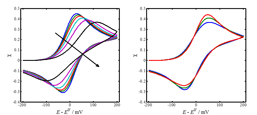
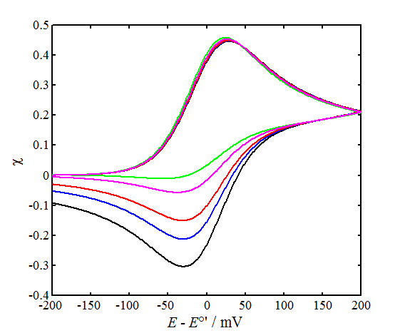
The left-hand panel of Figure 7.5 shows a few simulated voltammograms with varying values of parameter \( \psi \), keeping the scan limits and a constant. The peak separation \( \Delta E_p \) does not quite correspond to Table 7.1 because the smaller \( \psi \) is, the more sensitive is \( \Delta E_p \) to the switching potential where the scan direction is reversed.
In the right panel, parameter \( \psi \) is kept constant and the value of the charge transfer coefficient a is varied. As can be seen, the effect of \( \alpha \) on the shape of the voltammograms is rather small. Increasing \( \alpha \) increases the oxidation current peak and decreases the reduction current peak. Marcus theory showed that a is not a constant but varies slightly as the function of potential. The value 0.5 is therefore most commonly assumed to be \( \alpha \), which is quite an accurate assumption around the half-wave potential.
 |
|---|
|
Solving more complex reaction mechanisms is easier with
numerical simulations of the transport equations. Let us consider an EC mechanism
where R is first oxidized to O, which then reacts homogeneously further to P:
Let us assume that the electrochemical reaction is reversible and the homogeneous reaction is irreversible, with a rate constant of k. The transport equations are:
The equations above are converted into a dimensionless form with the following change of variables: \( C_i=c_i/c_{\text{R}}^b \), \( z=x/(D\tau) \) and \( T=t/\tau \); \( \tau \) is characteristic time of the measurement, e.g. the duration of the scan, t = 2|Ei – Es|/v. The transport equations now become
The continuity equation on the electrode becomes
The relationship between I(T) and c is easy to calculate when the scan limits, Ei and Es, are known. Equations (7.41) - (7.43) can be solved using various numerical methods.‡ A simulation with varying values of K can be found below
Figure 7.6 shows the characteristics of the EC mechanism:
when the rate of the homogeneous reaction increases or the scan rate decreases, the
reverse current vanishes because the oxidized species ‘O’ formed in the
electrochemical step reacts further to ’P’ to a greater extent, thereby decreasing
the concentration of ‘O’. Hence by measuring the reverse current peak at
varying scan rates, K can be
determined using a simulated working
curve. Such a working curve can represent, for example, the ratio of the
current peaks as a function of K[3].
|
|---|
If the peak separation \( \Delta E_p \) is less than 59/n mV, the electrode reaction is probably linked to an adsorption step. If adsorption is the rate-limiting step, the oxidation and reduction current peaks can be found at the same potential and are directly proportional to the scan rate, not to the square root of the scan rate like under diffusion control.
Electrode capacitance Cdl also contributes to the measured current. The capacitive (charging) current, iC, is
| \(\displaystyle i_c=C_{dl}v(1-e^{-t/RC_{dl}}) \) | (7.44) |
|---|
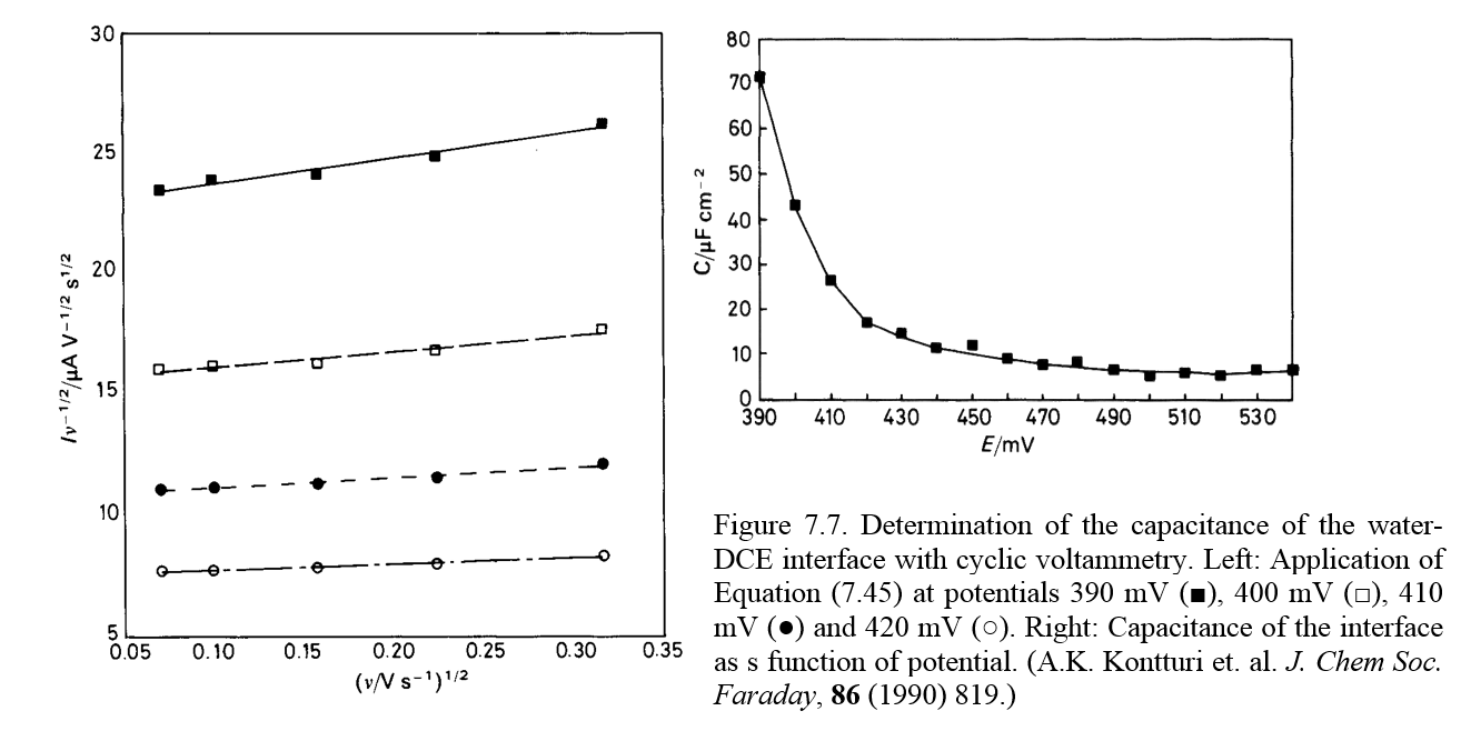
The exponential term of the above equation decays very fast. At solid electrodes, the contribution of the capacitive current is significant only at very high scan rates while at immiscible liquid-liquid interfaces it can be quite high. We derived above that the faradaic current is proportional to the square root of the scan rate. The total current iT is therefore
| \(\displaystyle i_{\text{T}}=A\sqrt{v}+C_{dl}v \Leftrightarrow i_{\text{T}}/\sqrt{v}=A+C_{dl}\sqrt{v} \) |
(7.45) |
|---|
where A is a constant. Plotting \( i_{\text{T}}/\sqrt{v} \) as a function of \( \sqrt{v} \) at each potential, a straight line is obtained with the slope of Cdl. Figure 7.7 shows just such an analysis of the water-1,2-dichloroethane (DCE) interface.
7.1.3. Current step
When constant current is fed to an electrode, the boundary condition of the transport problem is known, making the solution easy. Since the Laplace transform of the constant current density i is i/s, the surface concentrations in the Laplace domain are (only ’R’ initially present)
| \( \displaystyle\bar c_{\text{R}}(0,s)=\frac{c_{\text{R}}^b}{s}-\frac{i}{nF\sqrt{D_{\text{R}}}}\frac{1}{s^{3/2}} \) |
(7.46) |
|---|
| \(\displaystyle \bar c_{\text{O}}(0,s)=\frac{i}{nF\sqrt{D_{\text{O}}}}\frac{1}{s^{3/2}} \) |
(7.47) |
|---|
After inverse transformation,
| \( \displaystyle c_{\text{R}}(0,t)=c_{\text{R}}^b-\frac{2i\sqrt{t}}{nF\sqrt{\pi D_{\text{R}}}} \) | (7.48) |
|---|
| \( \displaystyle c_{\text{O}}(0,t)=\frac{2i\sqrt{t}}{nF\sqrt{\pi D_{\text{O}}}} \) |
(7.49) |
|---|
The moment when the surface concentration of ’R’drops to zero is known as the transition time, \( \tau \). It is given by the Sand equation:
| \( \displaystyle\sqrt{\tau}=\frac{nFc_{\text{R}}^b\sqrt{\pi D_{\text{R}}}}{2i} \) | (7.50) |
|---|
Surface concentrations can be written in a compact form with the transition time:
| \( \displaystyle c_{\text{R}}(0,t)=c_{\text{R}}^b\left(1-\sqrt{t/\tau}\right) \) |
(7.51) |
|---|
| \( \displaystyle c_{\text{R}}(0,t)=c_{\text{R}}^b \xi^{-1}\sqrt{t/\tau} \) | (7.52) |
|---|
|
Calculation of the concentration profiles does not pose a problem either. The profile of ’R’in the Laplace domain is
A comparison of Figures 7.1 and 7.8 reveals the fundamental difference between potential and current steps: potential step fixes the surface concentration and current step the concentration gradient at the surface as a constant. |
|---|
The electrode potential is obtained as a function of time applying Equations (7.51) and (7.52):
| \( \displaystyle E=E^{0'}-\frac{RT}{nF}\text{ln} [ \xi(\sqrt{\frac{\tau}{t}}-1) ] \) | (7.55) |
|---|
Transition time is therefore observed as the point at which the electrode potential changes abruptly. Times t = 0 and \( t=\tau \) are, in principle, singularities of Equation (7.55) but in practice this cannot naturally happen. At these points, something else than the redox couple being investigated defines the electrode potential after transition time, most probably the decomposition of the solvent.
Experimental determination of the transition time is not, however, simple. Since the experiment is not carried out under potential control, the electrode potential may drift before the transition time to the hydrogen (on the cathode) or oxygen evolution region (on the anode). The reduction of metals in particular is only easy on the mercury electrode that has an exceptionally high overpotential of hydrogen evolution.
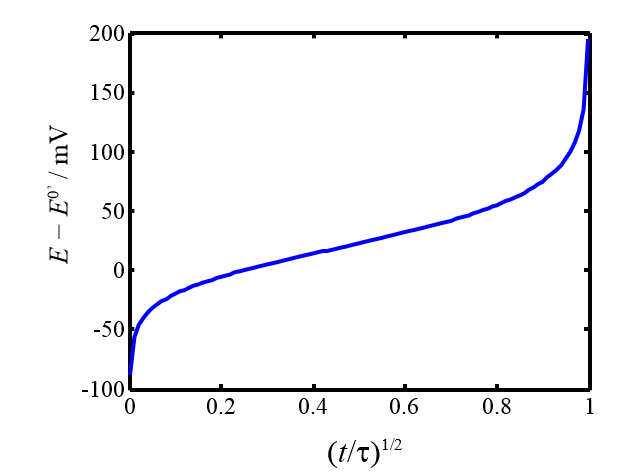
Figure 7.9. Electrode potential as a function of time during a current step experiment; n = 1 and \( \xi \) =1.
Electrode capacitance adds yet another level of difficulty. Capacitive current iC is defined as
| \( \displaystyle i_C=C_{dl}\frac{\partial E}{\partial t} \) | (7.56) |
|---|
Equation (7.56) means that a certain portion of the current is consumed by charging the electric double layer. Since the double layer capacitance Cdl is also a function of the electrode potential, this makes an accurate quantitative analysis of the effect of the capacitance rather difficult.
* The meaning of s is discussed in greater detail in the chapter on the impedance technique; it represents frequency.
† Function y = exp(x2)erfc(x) can be approximated with high accuracy with the polynomial y = 0.34802 z - 0.09587 z2 + 0.74785 z3, where z = (1 + 0.47047 x)-1. From: M. Abramowitz ja I.A. Stegun (Ed.), Handbook of Mathematical Functions, 7. p., Dover, New York, 1970, p. 299.
[1] R.S. Nicholson, I. Shain, Anal. Chem. 36 (1964) 7066.
[2] |Es - Ep| = 112.5/n mV. From: R.S. Nicholson, Anal. Chem. 37 (1965) 1351.
‡ See, e.g. D. Britz, Digital Simulation in Electrochemistry, 2. Ed., Springer, Berlin, 1988.
[3] A.K. Kontturi et al. J Electroanal. Chem. 418 (l996) 131.