CHEM-E4185 - Electrochemical Kinetics, 25.02.2019-29.05.2019
This course space end date is set to 29.05.2019 Search Courses: CHEM-E4185
Kirja
7. Electrochemical methods
7.2. Steady-state methods
In steady-state (or stationary) methods, the concentration does not change as a function of time, i.e. \( \partial c/\partial t =0 \), and Fick’s second law reduces into the form of \( \nabla^2c=0 \). This seems to simplify the solution of the transport problem, but this does not happen in practice because a true steady-state can only be reached without convection in spherical geometry. In this case, the operator \( \nabla^2 \) takes the form
| \( \displaystyle\nabla^2=\frac{\partial^2}{\partial r^2}+\frac{2}{r}\frac{\partial}{\partial r} \) (spherical geometry, no angular dependency) | (7.57) |
|---|
and the concentration profile is
| \( \displaystyle c(r)=A+\frac{B}{r} \) (spherical geometry, no angular dependency) | (7.58) |
|---|
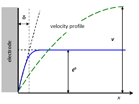
where A and B are constants. In linear geometry, in contrast, the concentration profile would be c(x) = A + Bx, but the boundary condition c(x→ ∞) = cb (or 0) would be absurd because the function A + Bx is not limited. In order to reach a true steady-state, the solution must be stirred resulting in an unstirred stagnant layer is forming on the surface of the electrode due to adhesion between the electrode and solvent molecules; we denote the thickness of this layer as \( \delta \). Now, the boundary condition changed to c(d) = cb (or 0), the transport problem has a meaningful solution in which the concentration changes linearly in the interval [0,\( \delta \)]. The real problem is determining the thickness \( \delta \).
Figure 7.10 shows how the thickness \( \delta \) is usually determined. The rate of the solution flow changes gradually from zero on the surface (non-slip condition) to its maximum value in the bulk. In channel flow, for example, the velocity profile is parabolic. The range of the velocity profile can be an order of magnitude wider than that of the concentration profile. According to Figure 7.10, \( \delta \) is defined as the thickness that is obtained by extrapolating the linear part of the concentration profile to the distance where the concentration would be equal to its bulk value. This is, however, only a thought, a virtual definition, because we cannot measure it. It is therefore evaluated from the solution of the transport problem using the measurable limiting current and assuming that in the region 0 < x < \( \delta \) there is no convection:
| \( \displaystyle c(x)=c^b-\frac{i(\delta-x)}{nFD} \Rightarrow \delta=\frac{nFDc_0}{i_{\text{lim}}} \) | (7.59) |
|---|
In this way, the Tafel slopes and (apparent) rate constant k0 could be determined, as described in Chapter 6, but in practice, steady-state methods are more sophisticated, taking convection explicitly into account via the solution of the convective diffusion equation
| \( \displaystyle D\nabla^2c-\vec{v}\nabla c=0 \) | (7.60) |
|---|
The solution velocity \( \vec{v} \) must be solved using the Navier-Stokes equation. These methods are therefore also known as hydrodynamic methods. [1] Because of the mathematical complexity of flow dynamics, only rotating disk and channel-flow electrodes are introduced in this book.
7.2.1 Rotating disc electrode (RDE)
When an electrode is rotated a velocity field is formed in its vicinity in a manner illustrated in Figure 7.11. The Navier-Stokes equation has been solved for this case in the form of a power series; we only need the first parabolic term in the series. The velocity profile perpendicular to the electrode surface is
| \( \displaystyle v(x)=-\frac{\omega^3}{v}^{1/2}0.510x^2=-Ax^2 \) | (7.61) |
|---|
where \( \omega \) is the angular frequency of rotation (\( \omega=2\pi f \)) and \( \nu \) is the kinematic viscosity of the solution (\( \eta/\ \rho \), for water ~0.01 cm2/s at 25 °C). At the electrode, the solution is thrown away from the center along the surface, but this velocity component does not contribute to the electric current: current is proportional only to the perpendicular component of the flux. Equation (7.61) also appears to give an absurd result that the velocity v(x) is increasing without limits with increasing distance x. First, the full solution with higher order series terms brings the velocity to zero at long distances and, second, Equation (7.61) applies only in the immediate vicinity of the electrode.
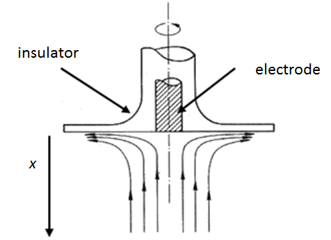
Figure 7.11. Solution flow near a rotating disk electrode.
|
Let us use equation (7.61) as the convection term in the Nernst-Planck equation:
Taking the divergence, the equation of convective diffusion is obtained:
The boundary conditions are c(\( x \rightarrow \infty \)) = cb, v(x=0) = 0, and the usual current boundary condition, Equation (3.48) [2]. Inserting p = dc/dx, the above equation becomes
The integral above can be calculated using the change of variables \( u=\frac{Ax^3}{3D} \Rightarrow dx=(\frac{D}{9A})^{1/3}u^{-2/3}du \). We therefore find the following:
where \( \Gamma \) is the Gamma function or the general factorial function; it is tabulated. It has the property \( \Gamma(m+1)=m\Gamma(m)=m! \). |
|---|
The limiting current density is obtained from Equation (7.66) setting c(x = 0) = 0:
The limiting current density is obtained from Equation (7.66) setting c(x = 0) = 0:
\( \displaystyle i_{\text{lim}}= \mp0.620nFD^{2/3}c^b\omega^{1/2}v^{-1/6} \) |
(7.68) |
|---|
The sign of the current must be chosen according to the reaction, i.e. if it is cathodic (i < 0) or anodic (i > 0). Equation (7.68) is known as the Levich equation and it tells us the important fact that ilim ~\( \omega \)1/2. Since all electrode reactions have a limited rate, an RDE is most suitable for the determination of reaction rate constants.
If current is measured at a potential where i < ilim, Equation (7.66) can be modified in the form of
| \(\displaystyle i=\frac{nFD(c^b-c(x=0))}{\delta} \) |
(7.69) |
|---|
where we have identified the thickness of the diffusion boundary layer \( \delta \) as the group of variables
| \( \displaystyle\delta=1.61D^{1/3}\omega^{-1/2}v^{1/6} \) | (7.70) |
|---|
Analogously to Chapter 6, we can again write the surface concentration as
| \( \displaystyle c(x=0)=c^b(1-i/i_{\text{lim}}) \) | (7.71) |
|---|
Let’s consider an oxidation reaction. Current density is i = nFkox cR(x=0) (only species ‘R’ initially present). Applying Equation (7.71) above, we get the following results:
| \( \displaystyle i=\frac{nFk_{ox}c_{\text{R}}^b}{1+(nFk_{ox}c_{\text{R}}^b)/i_{\text{lim}}} \) \( \displaystyle \frac{1}{i}=\frac{1}{nFk_{ox}c_{\text{R}}^b}+\frac{1}{0.620nFc_{\text{R}}^bD^{2/3}v^{-1/6}\omega^{1/2}}=\frac{1}{i_{\text{kin}}}+\frac{1}{i_{\text{lim}}} \) |
(7.72) |
|---|
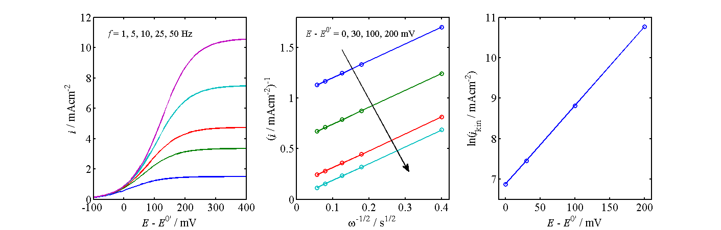
Figure 7.12. Determination of kinetics from the current-voltage curves of an RDE.
The analysis shown in Figure 7.12 proceeds as follows: At selected potentials, the inverse of current (density), i-1, is plotted as a function of \( \omega^{-1/2} \) and this line is extrapolated to zero, in other words to infinite angular frequency; the intercept gives the kinetic current density ikin and thereby kox. Kinetic current is the current that would occur in the absence of mass transfer limitations, ikin = nFkox cRb . A graph representing Equation (7.72) is commonly called as the Koutecký-Levich plot. As shown in the center panel of Figure 7.12, these lines should have the same slope at each potential. Finally, ln(ikin) is plotted as a function of the electrode potential. The slope of this line gives the charge transfer coefficient a, and the intercept at E = E0’ the value of k0.
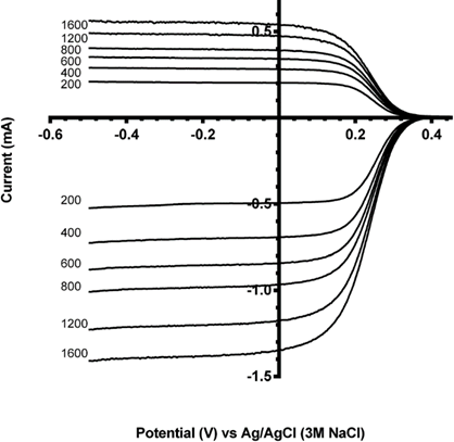
An RDE has an important modification, a rotating ring-disk electrode (RRDE) in which a concentric ring is placed around the disk at a distance of around 1 mm. Its purpose is to detect species on the ring that are formed on the disk. This can be accomplished, for example, by scanning the disk potential in the cathodic direction and keeping the ring at a constant anodic potential. Any reduced species on the disk are transported immediately to the ring (if they are soluble), where they can be re-oxidized. In this way, reaction mechanisms can be studied when the reaction intermediates are short-lived.
Calculus for the transport problem is rather challenging. An RRDE is calibrated by defining the collector efficiency with a known redox couple, i.e. finding the fraction of the species that is detected on the ring. The collector efficiency depends only on the electrode dimensions and the separation between the disk and the ring. An RRDE requires a bipotentiostat that is capable of controlling the disk and ring potential (or current) separately.
An example of RRDE calibration with a ferro/ferricyanide redox couple is shown below. On the glassy carbon disk, Fe3+ is reduced to Fe2+ whicht is then collected on the platinum ring. The numbers indicate the rotation rate in rpm. The ratio of the ring and disk current, in other words the collector efficiency N ≈ 41%.
7.2.2 Channel flow electrode
Another hydrodynamic method that has a wide practical use is the channel flow electrode. It is often used as a detector in liquid chromatography, capillary electrophoresis or flow injection analysis. The electrode is placed downstream in the flow channel, after a separation unit, and set at a sufficiently anodic or cathodic potential to oxidize or reduce the analyte on the electrode; it is therefore used under limiting current conditions. A reference electrode is usually placed upstream of the working electrode, while a counter electrode is preferably placed downstream of the working electrode in order to prevent its possible reaction products from being transported to the working electrode.
The transport problem of the channel flow electrode can be solved in a closed form for a rectangular channel because the velocity profile is accurately known. In a fully developed Poiseuille flow, the profile is parabolic with zero velocity on the channel walls that is known as the non-slip condition. The limiting current of a rectangular electrode is given by Equation (7.73), also known as the Levich equation:
| \( \displaystyle I_{lim}=0.925zFD^{2/3}c^bw\left(\frac{l^2\dot{V}}{h^2d}\right)^{1/3} \) | (7.73) |
|---|
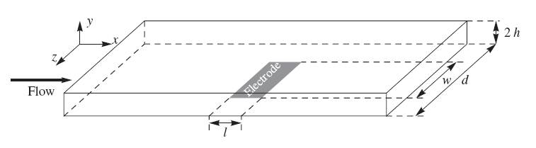
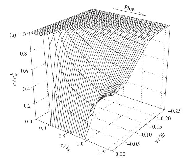
Figure 7.15. Concentration distribution near the channel flow electrode under limiting current conditions. From: Liljeroth et al., J. Electroanal. Chem., 483 (2000) 37.
The coefficient 0.925 in Equation (7.73) is sometimes replaced with 0.835, depending on the simplifying assumptions made in the derivation of the limiting current. The essential feature is, however, that the limiting current is proportional to the cubic root of the volume flow rate. In practice, the electrode response is calibrated using known concentrations, eliminating the significance of the constant coefficients. A detailed description of the solution of the transport problem is available in the literature [3] The problem is to solve first the Navier-Stokes equation and then the convective diffusion Equation (7.60). Figure 7.15 illustrates the concentration distribution of an analyte near the channel flow electrode, solved using the finite element method using Comsol Multiphysics® software. Although all transport problems can today be solved numerically without simplifying assumptions and in an arbitrary geometry, a closed form solution has the advantage that it provides the dependence of, say, the limiting current on the relevant variables explicitly.
[1] A classical textbook of hydrodynamic methods is: V.G. Levich, Physicochemical Hydrodynamics, Prentice Hall, Englewood Cliffs NJ, 1962.
[2] Think: why we are allowed to take the upper boundary condition at x → ∞, instead of x = d?
[3] K. Kontturi, L. Murtomäki, J.A. Manzanares, Ionic Transport Processes, Oxford University Press, 2009.