CHEM-E4185 - Electrochemical Kinetics, 25.02.2019-29.05.2019
This course space end date is set to 29.05.2019 Search Courses: CHEM-E4185
Kirja
7. Electrochemical methods
7.3. Ultramicroelectrodes
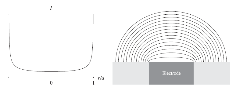
Figure 7.16. Radial current distribution (left) and equi-concentration lines (right) on a disk electrode.
As can be seen in Figure 7.16, the local current density increases very significantly towards the electrode edges. It can be shown that the radial distribution under mass transfer control is of the form
| \( \displaystyle i\propto\frac{1}{\sqrt{1-(r/a)^2}} \) | (7.74) |
|---|
where a is the disk radius. The current density is therefore in principle, unlimited at the edge r = a, but the integral over the disk remains limited. In reality, current density is kinetically limited at the edge of the disk. When the disk radius a is reduced down to a few microns, the concentration profile becomes nearly spherically symmetrical (see the right-hand panel of Figure 7.16), and Equation (7.57) can be used.
Ultramicroelectrodes are used in both transient and steady-state methods. In a steady-state, Equation (7.58) gives with the boundary conditions c(\( r \rightarrow \infty \)) = cb and c(r = a) = 0 the concentration profile
| \( \displaystyle c(r)=c^b(1-a/r) \) | (7.75) |
|---|
and the limiting current density
| \(\displaystyle i_{\text{lim}}=\pm nFD\left(\frac{dc}{dr}\right)_{r=a}=\pm nFD(c^b/a) \) | (7.76) |
|---|
If the electrode really were a hemisphere, the limiting current would be \( I_{\text{lim}}=\pm2\pi nFDc^ba \), but Fleischmann and Pons have shown [1] that the limiting current of a disk ultramicroelectrode is
| \( \displaystyle I_{\text{lim}}=\pm4nFDc^ba \) | (7.77) |
|---|
In practice, calculations are made in spherical geometry and the results are corrected as above.
In transient methods, the general Equation (7.4) takes the form
| \( \displaystyle\bar c_i(0,s)=\frac{c_i^b}{s}+ \frac{\bar i (s)}{nF\sqrt{D_i}(\sqrt{s}+\sqrt{D_i}/a)} \) | (7.78) |
|---|
proving that when \( a \rightarrow \infty \) the problem returns to linear geometry. Setting the surface concentration to zero, current density in a potential step experiment is in the Laplace domain
| \( \displaystyle\vec{i}(s)=\pm nF\sqrt{D}c^b\left(\frac{1}{\sqrt{s}}+\frac{1}{s}\frac{\sqrt{D}}{a}\right) \) | (7.79) |
|---|
After inverse transformation the result is
| \(\displaystyle i(t)=\pm nF\sqrt{D}c^b\left(\frac{1}{\sqrt{\pi t}}+\frac{\sqrt{D}}{a}\right) \) |
(7.80) |
|---|
Comparing this result with the Cottrell equation (7.11) of linear geometry, it is seen that the current density levels out after the transient period to Equation (7.76), contrary to the Cottrell equation in which the current decays to zero.
Figure 7.17. Current transients (7.76). For the Cottrell equation (7.11), \( \sqrt{D}/a=0 \).
Cyclic voltammograms of an ultramicroelectrode have an interesting feature that if the scan rate is low enough compared to the parameter D/a2, current is practically equal to that in a steady-state, like in Figure 6.3. When the scan rate is increased, the typical shape of a cyclic voltammogram, Figure 7.4, begins to emerge.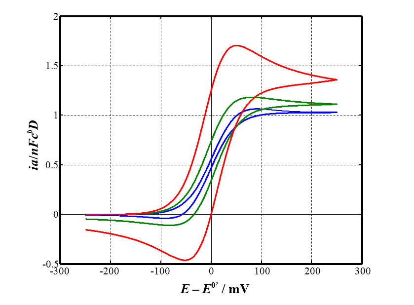
Figure 7.18. Cyclic voltammograms of an ultramicroelectrode at varying scan rates: v = 0.01 (blue), 0.1 (green) and 1.0 (red) Vs-1; electrode radius a = 10 \( \mu \)m.
[1] M. Fleischmann, S. Pons, in: D.R. Rolison, P.P. Schmidt (Eds.), Ultramicroelectrodes, Datatech Systems, Morganton, N.C., 1987.