CHEM-E4185 - Electrochemical Kinetics, 25.02.2019-29.05.2019
This course space end date is set to 29.05.2019 Search Courses: CHEM-E4185
Kirja
8. Impedance technique
Impedance technique or impedance spectroscopy is one of the essential methods in modern electrochemistry. It is conceptually very different from other electrochemical techniques and thus deserves its own chapter. In the impedance technique, only a very small periodic perturbation is applied either at equilibrium or in a steady-state, and the output signal caused by the input signal is measured as a function of frequency. A sinusoidal signal is generally used as an input, but in principle, you could also choose a triangular or square waveform input instead. A typical experimental arrangement of an impedance measurement is shown schematically in Figure 8.1.
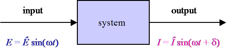
Figure 8.1. Principle of an impedance measurement.
When a voltage signal operating with angular frequency \( \omega \) and amplitude \( \hat{E} \) is applied, a current with an amplitude \( \hat{I} \) is produced in the system. The angular frequency of the signal remains constant while there is a phase shift \( \delta \) between the input and output signals. All the information about the system is included in the phase shift \( \delta \) and the ratio of the amplitudes \( \hat{Z}=\hat{E}/\hat{I} \) as a function of angular frequency.
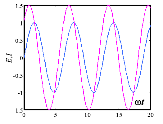
Presenting
data as a function of time as in Figure 8.2 is rather impractical and
pointless, since periodical signals repeat themselves and all the information
can be extracted from a single period (cycle). A sinusoidal signal
is therefore traditionally presented in terms of complex notation. Instead of the
notation in Figure 8.2, voltage and current can be expressed in polar
coordinates as
| \( \displaystyle E=\hat{E}e^{j\omega t} \) | |
| \(\displaystyle I=\hat{I}e^{j(\omega t+\delta)}
\) |
(8.1) |
|---|
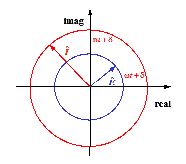
where j is imaginary, that is \( j=\sqrt{-1} \) [1]. Graphical representation of the complex notation is shown in Figure 8.3. The fundamental message of expressions (8.1) and Figure 8.3 is that the periodic signal does not change its value as a function of time, but is constant (\( \hat{E} \) or \( \hat{I} \)). However, its phase angle with respect to real axis, i.e. the projection to the real world, changes periodically as the vector rotates about the origin with an angular frequency \( \omega \).
The real and imaginary parts of the complex number z can be obtained from Euler’s formula:[2]
| \( \displaystyle z=\hat{z}e^{\pm j\varphi}=\hat{z}(\cos\varphi\pm j\sin\varphi) \) | (8.2) |
|---|
thus the sinusoidal signal is no more than the real part of a signal in the complex notation. Using Ohm’s law
| \( \displaystyle Z= \frac{E}{I} \) | (8.3) |
|---|
the complex impedance vector can be found to be
| \(\displaystyle Z=\frac{\hat{E}e^{j\omega t}}{\hat{I}e^{j(\omega t+\delta)}}=\frac{\hat{E}}{\hat{I}}e^{-j\delta}=\hat{Z}e^{-j\delta} \) | (8.4) |
|---|
The reciprocal of impedance Y = Z-1 is called admittance, and sometimes both of them combined are called immittance.
The message of equation (8.4) is very significant and profound: the time variable t has disappeared. The amplitude \( \hat{Z} \) and phase shift \( \delta \) depend only on the angular frequency \( \omega \), and thus the impedance of an electrochemical system must be calculated in the frequency domain instead of the time domain used in all other electrochemical methods. The time-dependent signal can be converted to the frequency domain using Laplace transform methods because the Laplace variable s is actually a complex number \( s=\sigma+j\omega \), but we have (arbitrarily) chosen \( \sigma=0 \).
|
In control systems engineering, all analyses are done in the Laplace domain. Let us denote the input in Figure 9.1 as U(s) and output as O(s). The relation between them is written as
where H(s) is the transfer function of a system, which tells us how the input signal is converted to the output signal by the system. The transfer function is a characteristic feature of a system, and thus U(s) can be arbitrary. The characteristics of a transfer function can be studied in the frequency domain by interpreting \( s=j\omega \). We therefore conclude analogously that the admittance Y of an electrochemical system is equal to its transfer function because according to Ohm’s law
If we choose a unit impulse as an input function, the output is equal to the transfer function because the Laplace transform of a unit impulse is U(s) = 1. |
|---|
Later in this chapter, we will present a method based on Laplace transformation that allows us to simplify the impedance analysis largely so that we do not have to write any of the periodic functions or any other forms of functions explicitly. However, some basic elements are easier to introduce using the complex notation as shown in the next subchapter.
[1] The symbol i usually stands for the imaginary unit, but now it is reserved for current density.
[2] More relations of complex numbers can be found
in 13.3. Relations of complex numbers.