CHEM-E4175 - Fundamental Electrochemistry, 09.01.2019-18.02.2019
This course space end date is set to 18.02.2019 Search Courses: CHEM-E4175
Kirja
2. Thermodynamics of electrolyte solutions
2.6. Osmosis
When a semi-permeable membrane separates two electrolyte solutions of different concentrations, osmotic pressure is created across the membrane. It should be emphasized that an ideal osmotic membrane is not permeable to any species other than water. Osmotic pressure is formed across an ion-selective membrane, but since no real membrane is ideal, the tiny amount of co-ions* in the membrane allows for slow diffusion of salt across the membrane, ultimately dissipating osmotic pressure. In biology, osmosis is an important issue but a cell membrane is not, strictly speaking, an osmotic membrane. Ionic concentrations are maintained by active membrane transporters.
Despite of the above critical comments, let us consider the emergence of osmotic pressure across an ideal osmotic membrane. Osmotic pressure is formed due to the imbalance of the chemical potential of water. Because only water can cross the membrane, the equilibrium condition of water at a constant temperature (dT = 0) between two aqueous phases α and β is written as
| \( \displaystyle\mu_1^{\alpha}\left(p,x_i^{ \alpha}\right)= \mu_1^{\beta}\left(p,x_i^{ \beta}\right) \) | (2.65) |
|---|
The chemical potential of water is therefore a function of the concentrations of all species and the pressures of the phases. (Subscript ’0’ is reserved for the solvent and the others for solutes.) The pressure dependence of the chemical potential is obtained using Equations (2.6) and (2.11) (note that the order of differentiation is free):
| \( \displaystyle\left(\frac{\partial\mu_i}{\partial p}\right)=\frac{\partial}{\partial p}\left(\frac{\partial G}{\partial n_i}\right)=\frac{\partial}{\partial n_i}\left(\frac{\partial G}{\partial p}\right)=\left(\frac{\partial V}{\partial n_1}\right)=\overline{V}_i \) | (2.66) |
|---|
where \( \overline{V_i} \) is the partial molar volume of species i. On the mole fraction scale
| \( \displaystyle d\mu_1=RTd\ln(f_1x_1)+\overline{V_1}dp \Rightarrow \mu_1=\mu_1^0+RT\ln(f_1x_1)+\overline{V_1}p \) | (2.67) |
|---|
Equation (2.67) is formally reached by an integration between pure water and a solution with the mole fraction x0 and activity coefficient f0 of water. Equilibrium between phases \( \alpha \) and \( \beta \) is therefore
| \( \displaystyle RT\ln(f_1^{\alpha}x_1^{\alpha})+\overline{V_1}^{\alpha}p^{\alpha}=RT\ln(f_1^{\beta}x_1^{\beta})+\overline{V_1}^{\beta}p^{\beta} \) | (2.68) |
|---|
Water is incompressible, and therefore its partial molar volume is constant unless the concentrations in the two solutions are very different. Osmotic pressure is:
| \( \displaystyle\pi=p^{\alpha}-p^{\alpha}=-\frac{RT}{\overline{V_1}}\ln\left(\frac{f_1^{\alpha}x_1^{\alpha}}{f_1^{\beta}x_1^{\beta}}\right) \approx-\frac{RT}{\overline{V_1}}\ln\frac{x_1^{\alpha}}{x_1^{\beta}} \) | (2.69) |
|---|
The ratio of the actitivy coefficients ≈ 1. Assume that phase β is pure water. Then
| \( \pi \approx -\frac{RT}{\overline{V_1}}\ln(x_1)=\frac{RT}{\overline{V_1}}\ln\left(1-\sum\limits_{k\neq1}x_k\right) \approx\frac{RT}{\overline{V_1}}\left(\sum\limits_{k \neq1}x_k\right) \) | (2.70) |
|---|
Because xk « x0 ≈ 1, xk ≈ nk /n0, and \( \overline V_1n_1 \approx V \) is the volume of the solution,
\( \pi \approx RT \sum\limits_{k}c_k \) |
(2.71) |
|---|
Equation (2.71) is known as the Van’t Hoff equation. Inserting, for example, c = 1.0 M = 1000 mol/m3, we see that \( \pi \) ≈ 24.5 atm (T = 298 K) corresponding to approximately 250 m height of a water column. This has led to the idea of a power plant that would harness osmotic pressure. An osmotic membrane is, however, very dense, making the flux of water very low. The power density hence remains very low, which makes such a power plant commercially unviable.
Equation (2.70) can be improved with an osmotic coefficient
| \( \displaystyle\pi=-\frac{RT}{\overline{V}}\ln(f_1x_1)=-\frac{\Phi RT}{\overline{V_1}}\ln (x_1) \Rightarrow \Phi-1=\frac{\ln f_1}{\ln x_1} \) | (2.72) |
|---|
that takes the unideality of a solution into account. Its values are tabulated for common electrolytes.
The correlation between the mean activity coefficient of an electrolyte and the osmotic coefficient is given without derivation in a binary system with the concentration c:
| \( \displaystyle d(c\Phi)=dc+c d\ln(\gamma_\pm) \Rightarrow\Phi=1+\frac{1}{c} \int_{0}^{c}{cd\ln\gamma_{\pm}} \) | (2.73) |
|---|
| \( \displaystyle d\ln\gamma_{\pm}=d\Phi+(\Phi-1)d\ln c \Rightarrow\ln\gamma_{\pm}=(\Phi-1)+ \int_{0}^{c}{(\Phi-1)} d\ln c \) | (2.74) |
|---|
If γ± is known in the concentration range [0,c], Φ can be calculated from Equation (2.73).
Accordingly, if the osmotic coefficient is measured in the same range, γ± can be calculated from (2.74). Measuring the mean activity coefficient
is relatively easy using electrochemical methods (electromotive force of a Galvanic
cell), and the osmotic coefficient can be evaluated from an experiment with an
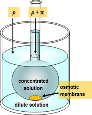
osmometer; the principle of such an experiment is depicted in Figure 2.6.
The Van’t Hoff equation can also be used to determine the molar mass of a macromolecule. Inserting a sample with mass m into the measurement chamber with the volume V, and measuring osmotic pressure, the molar mass M is obtained from the formula
| \( \displaystyle M=\frac{mRT}{\pi V} \) | (2.75) |
|---|
In biological experiments it is important to keep solutions isotonic, i.e. their osmocity equal to that of a living cell. Osmocity S is defined as the concentration of NaCl solution that has the same freezing point \( \Delta \)Tf as the solution being investigated. Osmolality O = ΔTf /Kf (Os/kg water) where Kf is the cryoscopic constant. ΔTf = -Kf m where m is the molality of a solute (≈ c). For water Kf = 1.86. The relation between the freezing point depression and osmotic pressure is (T = 273 K)
| \( \displaystyle\frac{\pi}{\text{atm}}=RT\frac{\Delta T_f}{K_f}=\frac{22.4}{1.86} \Delta T_f \cong12 \Delta T_f \) | (2.76) |
|---|
Equation (2.76) can be improved to also include the second term of the series expansion of Equation (2.70). In that case,
| \( \displaystyle\pi\cong12\Delta T_f-0.021(\Delta T_f)^2 \) atm | (2.77) |
|---|
Table 2.2 shows a few constants of freezing point depression and boiling point elevation for selected molecules; ΔTb = Kb m.
Table 2.2. Constants of freezing point depression and boiling point elevation for selected molecules. From: Handbook of Chemistry and Physics, 83. p. CRC Press, Boca Raton, 2002. With Publisher’s permission (CRC Press).
|
Substance |
Normal freezing point (K) |
Kf (K kg mol–1) |
Normal boiling point (K) |
Kb(K kg mol–1) |
|
Acetic acid |
289.6 |
3.59 |
391.2 |
3.08 |
|
Benzene |
278.6 |
5.12 |
353.3 |
2.53 |
|
Camphor |
449 |
40 |
482.3 |
5.95 |
|
Carbon disulfide |
161 |
3.8 |
319.2 |
2.40 |
|
Carbon tetrachloride |
250.3 |
30 |
349.8 |
4.95 |
|
Cyclohexane |
279.6 |
20.0 |
353.9 |
2.79 |
|
Ethanol |
158.8 |
2.0 |
351.5 |
1.07 |
|
Phenol |
314 |
7.27 |
455.0 |
3.04 |
|
Water |
273.15 |
1.86 |
373.15 |
0.51 |

| Example: The freezing point of blood serum is -0.53 °C. From Equation (2.77) we can calculate that its osmotic pressure \( \pi \) = 12.06×0.53 - 0.021×(0.53)2 atm ≈ 6.39 atm. The freezing point depression corresponds to approximately 0.53/1.86 ≈ 0.285 mol/kg NaCl solution. If a solution that is isotonic with serum is made from glucose, the glucose concentration should be approximately 88 g/dm3. Urea is frequently used in biochemistry: its required concentration would be only approximately 32 g/dm3 (values from the CRC table). The freezing point of a physiological solution (0.15 mol/kg NaCl) would be -0.28 °C, if calculated from the above equations. |
|---|
Quantities introduced in this paragraph are all colligative properties, i.e. the nature of the dissolved species does not, in principle, matter, only their concentration. A careful reader will note that osmotic coefficients are different for different electrolytes, which conflicts with the definition of the colligative properties. The theory presented above therefore only applies at moderately low concentrations.
* An ion with the opposite charge of the membrane is a counter-ion and an ion with the same charge a co-ion.
You can now test your conceptual knowledge by taking Quiz Chapter 2