CHEM-E4175 - Fundamental Electrochemistry, 09.01.2019-18.02.2019
This course space end date is set to 18.02.2019 Search Courses: CHEM-E4175
Kirja
3. Transport in electrolyte solutions
3.2. Concentration dependence of conductivity
The conductivity of a solution depends on the ionic concentrations, radii and viscosity of the solvent. Measuring the conductivity of the solution thus is – in principle – a simple means to determine ionic concentrations if molar conductivities are known, but there are a couple of problems. First, the above theory only concerns interactions between ions and solvent, i.e. it is valid in dilute solutions only. Second, an ionic radius in a solution is not an unambiguous quantity due to ion solvation. For example, the mobility of Li+ in water is lower than that of Na+, although its crystallographic radius is smaller. This is because Li+ is so strongly hydrated that it drags a mantle of water with it during transport. Polyatomic ions such as sulphate are not completely spherical either.
Nevertheless, measuring conductivity is one of the oldest electrochemical measurements, and data is available for common electrolytes in a wide range of concentrations and temperatures in aqueous solutions. The division of electrolytes into strong and weak ones, and classical theories of electrolytes are based on this experimental data.
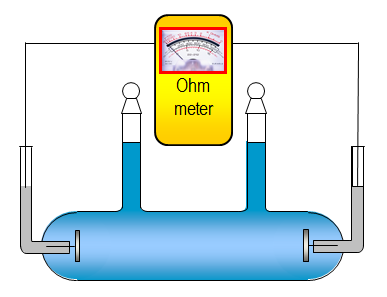
Conductivity is measured with AC current in order to prevent concentration polarization. The electrodes are usually porous platinum plates to minimize the resistance that may occur as a result of electrode reactions. The measured resistance of a conductivity cell (Figure 3.3), Rs is
| \( \displaystyle R_s= \frac{1}{\kappa} \frac{l}{A} \) | (3.21) |
|---|
The geometric cell constant A/l is evaluated using a solution with known conductivity, usually 1.0 mM KCl.
3.2.1 Strong electrolytes
Ion-ion interaction is very strong compared with other intermolecular forces. It is inversely proportional to distance while, van de Waals interaction, for example, is inversely proportional to the sixth power of distance. Typical electrostatic energy between two ions can be as high as 250 kJ mol-1, which is of the order of the energy of a covalent bond, while the energy of a hydrogen bond is only approximately 10-40 kJ mol-1. Coulombic forces may cause some extra trouble in molecular dynamics simulations of electrolytes because it is not sufficient to compute the interactions with the neighboring molecules only but computation must be extended over several layers of molecules. Periodical boundary conditions are often needed because electrostatic forces can stretch over the limits of the simulation domain.
Due to coulombic interactions the activity coefficients of electrolytes deviate from unity even in rather dilute solutions. For the same reason, ionic molar conductivity also very much depends on the concentration. The concentration dependence of a diffusion coefficient is obtained as (see paragraph 3.3)
| \( \displaystyle D_i=D_{i,\infty}\left(1+ \frac{\partial\text{ln}\gamma_i}{\partial\text{ln}c_i}\right) \) | (3.22) |
|---|
where Di,∞ is the diffusion coefficient at infinite dilution. The dependence of an activity coefficient on the concentration is given by the Debye-Hückel theory. Using the limiting law
| \( \text{log}\gamma_{\pm}=z_+z_- A\sqrt{I} \) | (3.23) |
|---|
For a 1:1 electrolyte (I = c = ci):
| \( \displaystyle \frac{\partial\text{ln}\gamma_i}{\partial\text{ln}c_i}=c\frac{\partial\text{ln}\gamma_i}{\partial c}=- \frac{1}{2}A \sqrt{c} \) | (3.24) |
|---|
| \( \displaystyle D_i=D_{i, \infty}\left(1- \frac{2.303}{2}A \sqrt{c}\right) \) | (3.25) |
|---|
Molar conductivity of an electrolyte,
Λ, is the sum of ionic conductivities,
| \( \Lambda= \upsilon_+\ \lambda_++ \upsilon_-\ \lambda_- \). | (3.26) |
|---|
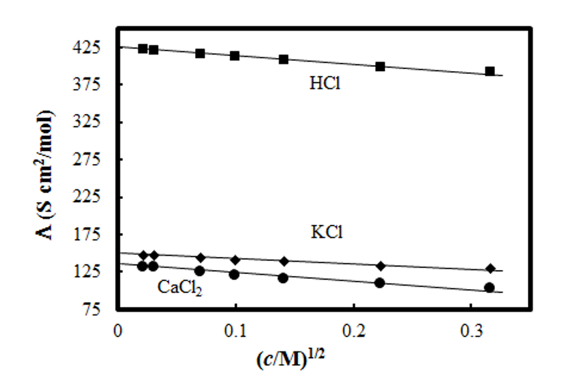
Hence, combining Equations (3.16), (3.25) and (3.26) Kohlrausch's law is achieved,
| \( \Lambda= \Lambda_{ \infty}-K\sqrt{c} \), | (3.27) |
|---|
which is experimentally verified in relatively dilute solutions (c < 0.1 M). Since K includes the product z+z− it is the same for all salts of the same type, see Figure 3.4. Measuring \( \Lambda \) at varying concentrations and extrapolating to infinite dilution, \( \Lambda_ \infty \)can be determined. Combining this data with transport numbers that are discussed later on, ionic molar conductivities at infinite dilution, λi,∞, can be evaluated. Tables of these can be found in several textbooks of physical chemistry.
3.2.2 Weak electrolytes
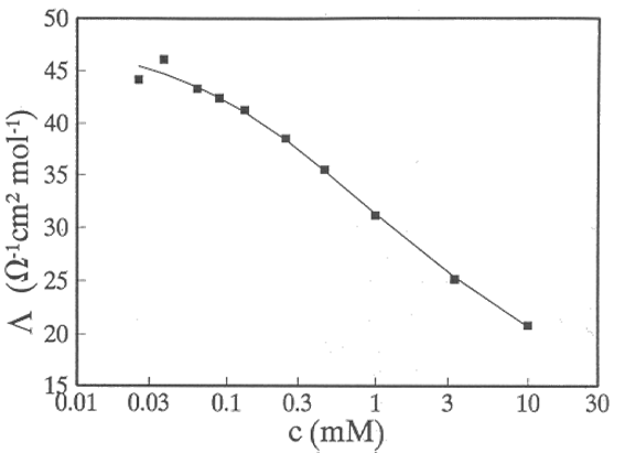
The conductivity of weak
electrolytes that only partially dissociate to free ions follows a different kind
of dependence on the concentration (see paragraph 2.5.2 for a discussion of
dissociation). Since the degree of dissociation, \( \alpha \), is often quite low, the concentrations of free
ions also remain low, and their molar conductivities are practically equal to
the values at infinite dilution. For a 1:1 electrolyte the conductivity \( \kappa \) is
| \( \kappa= \alpha c( \lambda_{+, \infty}+ \lambda_{-, \infty})=\alpha c \Lambda_{ \infty} \) | (3.28) |
|---|
and therefore
| \( \displaystyle \alpha= \frac{\Lambda}{\Lambda_ \infty} \) | (3.29) |
|---|
Arranging the expression of the dissociation constant Kd = α2c/(1 – α) in the form of
| \( \displaystyle\frac{1}{\alpha}=1+\frac{\alpha c}{K_d} \Rightarrow \frac{1}{\Lambda}=\frac{1}{\Lambda_{\infty}}+\frac{\Lambda c}{K_d\Lambda_\infty^2}\) | (3.30) |
|---|
a plot of Λ-1 vs. Λc = κ is linear with the intercept \( \Lambda_ \infty^{-1} \) on the y axis; Kd can be calculated from the slope. Equation (3.30) is known as Ostwald's dilution law; it applies relatively well in aqueous solutions.
In organic solvents, electrolyte dissociation is nearly always incomplete. Constants A and B in the Debye-Hückel theory include the relative permittivity of the solvent εr (previously called the dielectric constant). Calculating their values it transpires that even at low ionic strengths (c < 10-3 M) the mean activity coefficient deviates from unity. Ostwald's dilution law therefore does not apply as such but the activity coefficients need to be retained in the analysis.
Molar conductivity can be written in the form of (1:1 electrolyte)
| \( \Lambda=\alpha(\Lambda_\infty-K\sqrt{\alpha c}) \) | (3.31) |
|---|
Solving \( \alpha \) from the expression of Kd (Equation (2.45)) gives:
| \( \displaystyle\alpha=\frac{K_d(\sqrt{1+4\gamma_{\pm}^2c/K-d}-1}{2\gamma_{\pm}^2c} \) | (3.32) |
|---|
[1] Large number conductivity measurements in varying solution composition with the above analysis is given by R.M. Fuoss et al., J. Soln. Chem. 3 (1974) 45; 4 (1975) 91; 4 (1975) 175.