CHEM-E4175 - Fundamental Electrochemistry, 09.01.2019-18.02.2019
This course space end date is set to 18.02.2019 Search Courses: CHEM-E4175
Kirja
6. Electrochemical reaction kinetics
6.2. Current-voltage curves
\( \displaystyle\frac{i}{nF}=k_{ox}c_{\text{R}}^s-k_{red}c_{\text{O}}^s \) |
(6.12) |
|---|
Inserting the dependence of the rate constants on potential it is therefore possible to sketch a current-voltage curve; the only problem comes from the surface concentrations that change as a function of electric current. We begin the analysis with a reversible reaction, i.e. a reaction that has such a high rate that the surface concentrations follow the Nernst equilibrium at all times and in all currents.
6.2.1 Reversible reaction
We consider only the case of a trace ion (see (3.47)) that gives the boundary condition
| \(\displaystyle\frac{i}{nF}=D_{\text{R}}\left(\frac{\partial c_{\text{R}}}{\partial x}\right)_{x=0}=-D_{\text{O}}\left(\frac{\partial c_{\text{O}}}{\partial x}\right)_{x=0} \) | (6.13) |
|---|
In a stationary state (steady state) the diffusion equation (3.53) becomes
| \( \displaystyle\frac{\partial c}{\partial t}=D\frac{\partial^2c}{\partial x^2}=0 \) | (6.14) |
|---|
making concentration profiles linear. As will be explained in Chapter 7, a diffusion boundary layer (DBL) of the thickness \( \delta \) is formed in the vicinity of an electrode. With the boundary condition \( c_i(\delta)=c_i^b(i=\text{R,O}) \) the following result is reached:
| \( \displaystyle\frac{i}{nF}=D_{\text{R}}\frac{c_{\text{R}}^b-c_{\text{R}}^s}{\delta}=D_{\text{O}}\frac{c_{\text{O}}^b-c_{\text{O}}^s}{\delta} \) | (6.15) |
|---|
In Figure 6.2, steady-state concentration profiles during an oxidation reaction are depicted (anodic current, i > 0).
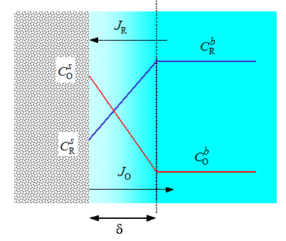
It should be noted that the fluxes of O and R are equal but opposite in direction, JR = -JO, in order to maintain the mass balance, as Equation (6.13) actually also shows. As can easily be seen from the picture, (and Equation (6.15) the highest possible current is obtained when the surface concentration of R reaches zero. This current is called the limiting current. Accordingly, if we consider a reduction reaction, the highest possible cathodic current (i < 0) is obtained when the surface concentration of O reaches zero. The anodic and cathodic current densities are respectively obtained from Equation (6.15):
| \( \displaystyle i_{\text{lim}}^{ox}=nFD_{\text{R}}c_{\text{R}}^b/\delta \) and \( i_{\text{lim}}^{red}=-nFD_{\text{O}}c_{\text{O}}^b/\delta \) |
(6.16) |
|---|
The surface concentrations can be written with the help of current density as:
| \( \displaystyle c_{\text{R}}^s=c_{\text{R}}^b-\frac{i\delta}{nFD_{\text{R}}} \) and \( c_{\text{O}}^s=c_{\text{O}}^b+\frac{i\delta}{nFD_{\text{O}}} \) |
(6.17) |
|---|
From Equation (6.16), the bulk
concentrations can be solved as a function of the limiting current density, as a result of which the following very useful expressions are obtained:
| \( \displaystyle c_{\text{R}}^s=\frac{\left(i_{\text{lim}}^{ox}-i\right)\delta}{nFD_{\text{R}}} \) and \( c_{\text{O}}^s=-\frac{\left(i_{\text{lim}}^{red}-i\right)\delta}{nFD_{\text{O}}} \) |
(6.18) |
|---|
| \( \displaystyle c_{\text{R}}^s=c_{\text{R}}^b\left(1-\frac{i}{i_{\text{lim}}^{ox}}\right) \) and \( c_{\text{O}}^s=c_{\text{O}}^b\left(1-\frac{i}{i_{\text{lim}}^{red}}\right) \) |
(6.19) |
|---|
Equation (6.18) or (6.19) cannot naturally be written for a species that has zero bulk concentration. For example, if \( c_{\text{O}}^b=0 \), current is always positive and
| \( \displaystyle c_{\text{O}}^s=\xi^{-2}c_{\text{R}}^b\frac{i}{i_{\text{lim}}^{ox}} \) ; \( \xi^2=\frac{D_{\text{O}}}{D_{\text{R}}} \) |
(6.20) |
|---|
Using Equation (6.18), the Nernst equation can be written in a form that makes the simulation of the current-voltage curve very simple:
\( \displaystyle E=E^{0'}-\frac{RT}{nF}\text{ln}(\xi^2)+\frac{RT}{nF}\ln\left(\frac{i-i_{\text{lim}}^{red}}{i_{\text{lim}}^{ox}-i}\right) \) |
(6.21) |
|---|
 |
 |
|---|
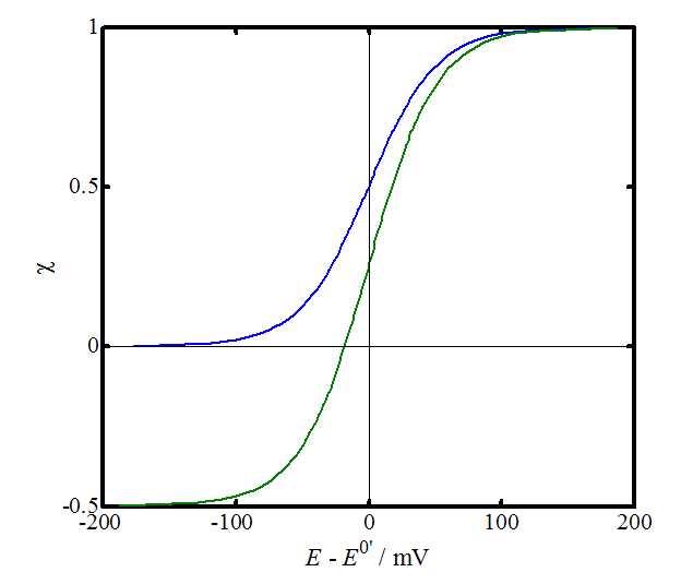
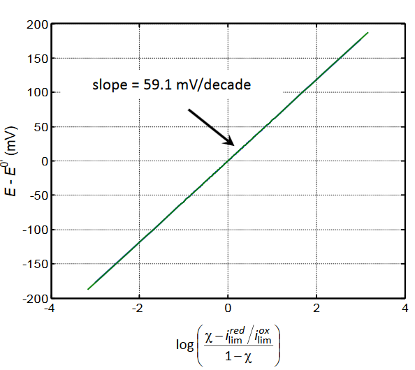
Figure 6.3 shows current-voltage curves with \( i_{\text{lim}}^{red}/{i_{\text{lim}}^{ox}}=0 \) or -0.5 and n = 1. The diffusion coefficients are usually rather close to one another, hence \( \xi^2 \approx1 \). Scaled current density \( \chi \) is defined as \( \chi=i/i_{\text{lim}}^{ox} \). Equation (6.21) provides a diagnostic criterion for a reversible electrode reaction: plotting the electrode potential as a function of the logarithm on the right-hand side of Equation (6.21), a straight line is obtained with a slope of 25.7/n mV, or on the log10 scale, 59.1/n mV per decade.
6.2.2 Quasi-reversible reaction
The derived equations above (6.15)-(6.19) are generally valid and can be used in Equation (6.12) to simulate current-voltage curves. Inserting Equation (6.17), for example, we find that
| \( \displaystyle \frac{i}{nF}=\frac{k_{ox}c_{\text{R}}^b-k_{red}c_{\text{O}}^b}{1+\frac{k_{ox}\delta}{D_{\text{R}}}+\frac{k_{red}\delta}{D_{\text{O}}}} \) | (6.22) |
|---|
In practice, the curves are preferably presented in terms of measurable quantities. The determination of the thickness of the DBL, \( \delta \), for example, is not unambiguous, as will be seen in Chapter 7.
Let us consider equilibrium again. Now, kred,eq cOb = kox,eq cRb because in the absence of electric current there is no concentration polarization, and surface concentrations are equal to bulk ones. At equilibrium, the rate of oxidation is equal to the rate of the reduction; they are not zero but the equilibrium is a dynamic process where the net reaction rate is zero. The Nernst equation is valid at equilibrium:
| \( \displaystyle\frac{c_{\text{O}}^b}{c_{\text{R}}^b}=e^{nf(E_{eq}-E^{0'})} \) | (6.23) |
|---|
Inserting the above equation into the expression of kred in Equation (6.10), we find that
| \( \displaystyle k_{red,eq}=k^0\left(\frac{c_{\text{O}}^b}{c_{\text{R}}^b}\right)^{\alpha-1} \) | (6.24) |
|---|
Exchange current density, i0, is defined as the inherent rate of oxidation or reduction at equilibrium:
\(\displaystyle i_0=nFk_{red,eq}c_{\text{O}}^b=nFk^0 c_{\text{O}}^b\left(\frac{c_{\text{O}}^b}{c_{\text{R}}^b}\right)^{\alpha-1}=nFk^0\left(c_{\text{O}}^b\right)^{\alpha}\left(c_{\text{R}}^b\right)^{1-\alpha} \) |
(6.25) |
|---|
Exchange current density is the measure of the rate of an electrode reaction, i.e. of its reversibility. A good reference electrode, such as Ag/AgCl has an exchange current as high as 10 A/cm2. Such an electrode is ideally non-polarizable, as discussed in Chapter 1.
The definition of overpotential is \( \eta=E-E_{eq} \). Hence, \( E-E^{0'}=E-E_{eq}+E_{eq}-E^{0'}= \eta+E_{eq}-E^{0'} \). The current-overpotential equation can be derived by applying Equation (6.23) to the last equality:
| \( \displaystyle\frac{i}{nF}=c_{\text{R}}^sk^0e^{\alpha nf\eta}\left(\frac{c_{\text{O}}^b}{c_{\text{R}}^b}\right)^{\alpha}-c_{\text{O}}^sk^0e^{(\alpha-1)nf\eta}\left(\frac{c_{\text{O}}^b}{c_{\text{R}}^b}\right)^{\alpha-1}=k^0(c_{\text{O}}^b)^{\alpha}(c_{\text{R}}^b)^{1-\alpha}\left[\frac{c_{\text{R}}^s}{c_{\text{R}}^b}e^{\alpha nf\eta}-\frac{c_{\text{O}}^s}{c_{\text{O}}^b}e^{(\alpha-1) nf\eta}\right] \) | (6.26) |
|---|
\( \displaystyle\frac{i}{i_0}=\frac{c_{\text{R}}^s}{c_{\text{R}}^b}e^{\alpha nf\eta}-\frac{c_{\text{O}}^s}{c_{\text{O}}^b}e^{(\alpha-1) nf\eta} \) |
(6.27) |
|---|
If the solution is stirred effectively or the current is less than 10% of the limiting current, the concentration polarization can be ignored, and the Butler-Volmer equation is obtained*:
| \( \displaystyle\frac{i}{i_0}=e^{\alpha nf\eta}-e^{(\alpha-1) nf\eta} \) | (6.28) |
|---|
The above equation is traditionally analyzed at limiting values of overpotential. At low overpotentials it can be linearized, giving
| \( \displaystyle i \approx i_0\frac{nF}{RT} \eta \Rightarrow \eta=\frac{RT}{nFi_0}i \) | (6.29) |
|---|
The unit of the group of variables RT/(nFi0) is \( \Omega \text{cm}^2 \); it is known as the charge transfer resistance, Rct.
At high positive overpotentials, only the anodic term of Equation (6.28) is significant. Hence
| \(\displaystyle \eta=-\frac{RT}{\alpha nF}\text{ln}i_0+\frac{RT}{\alpha nF}\text{ln}i \) |
(6.30) |
|---|
Accordingly, at high negative overpotentials only the cathodic term is significant:
| \( \displaystyle\eta=-\frac{RT}{(1-\alpha)nF}\text{ln}i_0+\frac{RT}{(\alpha-1)nF}\text{ln}|i| \) | (6.31) |
|---|
Equations (6.30) and (6.31) are called Tafel equations. The graphs of ln| i | vs. \( \eta \) are linear, and their extrapolation to zero overpotential gives the value of i0. This kind of a graph is called a Tafel plot. The original Tafel equation was empirical and written as
| \( \displaystyle\eta=a+b\log i \) | (6.32) |
|---|
where a and b were experimental constants; b is known as the Tafel slope. Comparing Equations (6.31) and (6.32), the cathodic Tafel slope is†
| \(\displaystyle b=\frac{2.303RT}{(\alpha-1)nF} \) | (6.33) |
|---|
Very often n = 1 and \( \alpha \approx0.5 \), giving a typical Tafel slope of approximately 120 mV per current decade. If mass transfer to the electrode is inefficient, the linear range of the plot can be rather limited due to concentration polarization, making the determination of Tafel slopes difficult. Measurements are therefore most often carried out with a rotating disk electrode (see Chapter 7.2.1), which makes the explicit elimination of mass transfer possible.
In a complete current-overpotential curve, mass transfer is taken into account. Inserting Equations (6.19) into Equation (6.27) the following expression can be derived:
| \( \displaystyle\chi=\frac{e^{\alpha nf\eta}-e^{(\alpha-1) nf\eta}}{\chi_{\text{kin}}+e^{\alpha nf\eta}+\chi_{\text{lim}}e^{(\alpha-1) nf\eta}} \) ; \( \chi_{\text{kin}}=\frac{i_{\text{lim}}^{ox}}{i_0} \) ; \( \chi_{\text{lim}}=\frac{i_{\text{lim}}^{ox}}{i_{\text{lim}}^{red}} \) |
(6.34) |
|---|
\( \chi \) is defined similarly to Figure 6.3, \( \chi=i/{i_{\text{lim}}^{ox}} \).
Figure 6.4 presents simulated curves using Equation (6.34). It shows the effect of the exchange current density: the lower it is, i.e. the higher \( \chi_{\text{kin}} \) is, the wider the potential range where hardly any current flows (potential window). At the limit i0 → 0 an electrode is ideally polarizable and its i-h graph horizontal. As discussed earlier, an ideally non-polarizable electrode has a very high exchange current density and without mass transfer limitations, its \( i-\eta \) graph would be vertical. In Figure 6.4, the curve with \( \chi_{\text{kin}}=0.1 \) is already completely under mass transfer control because with values lower than that the shape of the curve no longer changes.
An ideally non-polarizable electrode naturally cannot exist because solvent decomposes at high overpotentials. A mercury electrode is closest to an ideally polarizable electrode because the overpotential of hydrogen evolution (see paragraph 6.5.2) on mercury is very high, expanding the potential window over 2 V. Immiscible water-organic interfaces are also polarizable, although the potential window usually remains less than 1 V.
Figure 6.4. Simulated i-\( \eta \) curves with \( \chi \)kin = 0.1 -104, \( \alpha \) = 0.5, n = 1 or 2 and \( \chi \)lim = 2.
* The theory presented in this chapter is commonly called the Butler-Volmer theory and Equation (6.12) the Butler-Volmer equation, although it originally meant Equation (6.28).
† In an old polarographic convention, cathodic current was positive and, therefore, the current has no sign.