CHEM-E4175 - Fundamental Electrochemistry, 09.01.2019-18.02.2019
This course space end date is set to 18.02.2019 Search Courses: CHEM-E4175
Kirja
8. Impedance technique
8.3. Determining the impedance of an electrochemical system
We have previously stated that impedance is a frequency-dependent quantity and therefore the most convenient and reasonable way to determine it is in the frequency domain. The conversion from a time variable to a frequency variable is done using Laplace transformation, and because of this, we start with a couple of important remarks concerning Laplace transforms [1]. The Laplace transform is a linear operator:
| \( \mathcal{L}\{af(t)+bg(t)\}=a\mathcal{L}\{f(t)\}+b\mathcal{L}\{g(t)\}=a\overline{F}(s)+b\overline{G}(s) \) |
|
| \( \mathcal{L}\{f(t)g(t)\} \neq \mathcal{L}\{f(t)\}\mathcal{L}\{g(t)\} \) |
(8.14) |
|---|
The symbol \( \mathcal{L} \) represents the Laplace transform, a and b are constants, and f(t) and g(t) arbitrary functions of time; \( \overline{F}(s) \) and \( \overline{G}(s) \) are transforms of f(t) and g(t). The bar over the function highlights the frequency domain and s is the Laplace variable (frequency).
The
transform being linear means that non-linear factors, such as product kf cs cannot be
converted (kf is a
potential dependent rate constant and cs
surface concentration of the reacting species). Non-linear factors therefore have to
be linearized near measurement potential, and because of this, the magnitude of
the input signal has to be small enough for a valid linearization. A few
examples of the most common linearizations are shown in the following
subchapters. Impedance of any given system can be determined following the
steps below:
|
1. Linearize the current-voltage equation. 2. Solve the problem in Laplace domain. 3. Remove non-periodical components of the solution with the relation
4. Impedance is \(\displaystyle Z=\frac{E(j\omega)}{I(j\omega)} \) |
|---|
The third step deserves a couple of remarks. The Laplace transform of a sinusoidal signal takes the form \( 1/(s^2+\omega^2) \), so multiplication with a binomial \( (s^2+\omega^2) \) removes the denominator. All other signals without such a denominator approach zero at the limit \( s=j\omega \). Actually, there is no need to apply Equation (8.15) in practice because all terms without \( \overline{E}(s) \)or \( \overline{I}(s) \) can be eliminated. The following examples will clarify the method.
8.3.1 Linearization of current-voltage curves and faradaic impedance
Current-overpotential equation (6.27) was derived in Chapter 6:
| \( \displaystyle\frac{i}{i_0}=\frac{c_{\text{R}}^s}{c_{\text{R,0}}^b}e^{\alpha nf\eta}-\frac{c_{\text{O}}^s}{c_{\text{O,0}}^b}e^{(\alpha-1) nf\eta} \) | (6.27) |
|---|
Let us linearize this equation at the point of equilibrium \( (i=0, \eta=0, c_{\text{R}}^s=c_{\text{R,0}}, c_{\text{O}}^s=c_{\text{O,0}}) \):
| \( \displaystyle\left(\frac{\partial(i/i_0)}{\partial c_{\text{R}}^s}\right)_{eq}=\frac{1}{c_{\text{R}}^b} ;\left(\frac{\partial(i/i_0)}{\partial c_{\text{O}}^s}\right)_{eq}=-\frac{1}{c_{\text{O}}^b} \) | (8.16) |
|---|
| \( \displaystyle\left(\frac{\partial(i/i_0)}{\partial\eta}\right)_{eq}=\alpha f-(\alpha-1)f=f \) |
|
| \( \displaystyle\frac{i}{i_0} \approx\frac{c_{\text{R}}^s-c_{\text{R,0}}}{c_{\text{R,0}}} -\frac{c_{\text{O}}^s-c_{\text{O,0}}}{c_{\text{O,0}}}+f\eta=\frac{c_{\text{R}}^s}{c_{\text{R,0}}}-\frac{c_{\text{O}}^s}{c_{\text{O,0}}}+f\eta \) |
(8.17) |
|---|
Equation (8.17) can be written directly in the
Laplace domain as follows:
| \( \displaystyle\overline{\eta}(s)=\frac{RT}{nF}\left(\frac{\overline{i}(s)}{i_0}-\frac{\overline{c}_{\text{R}}^s(s)}{c_{\text{R,0}}}+\frac{\overline{c}_{\text{O}}^s(s)}{c_{\text{O,0}}}\right) \) | (8.18) |
|---|
Now we need to determine the surface
concentrations \( \overline{c}_{\text{R}}^s(s) \) and \( \overline{c}_{\text{O}}^s(s) \) from the
transfer equations, which we already did in Chapter 7. Substituting
Equations (7.7) and (7.8) to Equation (8.18) gives
| \( \displaystyle\overline{\eta}(s)=\frac{RT}{nF}\left(\frac{\overline{i}(s)}{i_0}+\frac{\overline{i}(s)}{nFc_{\text{R,0}}\sqrt{sD_{\text{R}}}}+\frac{\overline{i}(s)}{nFc_{\text{R,0}}\sqrt{sD_{\text{O}}}}\right) \) | (8.19) |
|---|
Dividing Equation (8.19) by \( \overline{i}(s) \) and replacing s with \( j\omega \), impedance can easily be found:
| \( \displaystyle Z=\frac{RT}{nFAi_0}+\frac{RT}{n^2F^2A}\left(\frac{1}{c_{\text{R,0}}\sqrt{D_{\text{R}}}}+\frac{1}{c_{\text{O,0}}\sqrt{D_{\text{O}}}}\right)\frac{1}{\sqrt{j\omega}} \) | (8.20) |
|---|
Note that because i stands for current density, we needed to divide the expression by
the area A. The first term of
Equation (8.20) represents charge transfer resistance, Rct. The rate constant of the reaction, k0, can be
determined by substituting the expression for the exchange current density in
Equation (8.20). The latter term of the equation is known as the Warburg element,
which describes diffusion. Because \( j^{1/2}=(1-j)/\sqrt{2} \), it is evident
that the real and imaginary parts of the Warburg element are equal. The
faradaic impedance of the electrode reaction, Zf, is therefore
| \( \displaystyle Z_f=R_{ct}+\frac{\sigma}{\sqrt{\omega}}(1-j) \) | (8.21) |
|---|
where \( \sigma \) is the Warburg element
| \( \displaystyle\sigma=\frac{RT}{n^2F^2A\sqrt{2}}\left(\frac{1}{c_{\text{R,0}}\sqrt{D_{\text{R}}}}+\frac{1}{c_{\text{O,0}}\sqrt{D_{\text{O}}}}\right) \) |
(8.22) |
|---|
The characteristic feature of Warburg
impedance is an increasing straight line at an angle of 45 degrees. When
faradaic impedance and electrode capacitance are in parallel and the solution
resistance is added in front of the whole circuit, an impedance plot shown in
Figure 8.9 is obtained. The whole circuit is called the Randles circuit or Randles
equivalent circuit, shown in Figure 8.11.
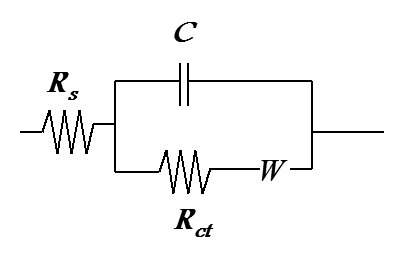
Figure 8.9 shows how the values for Rs and Rct can easily be obtained. The semicircle and the straight line are usually overlapping, so only the left-hand side (high frequencies) of the semicircle is visible. Despite this, it is easy to determine the numerical values using modern software; we will come back to the fitting of circuit components later in this Chapter.
If the solution resistance and capacitance have been eliminated from the experimental data, the residual faradaic impedance can be divided into real and imaginary parts:
| \( \displaystyle Z_f'=R_{ct}+\sigma/\sqrt{\omega} \) |
|
| \( \displaystyle Z_f''=\sigma/\sqrt{\omega} \) |
(8.23) |
|---|
Plotting the real and imaginary parts as a function of \( 1/\sqrt{\omega} \), two straight lines are obtained. Of these two, the real part intersects the vertical axis at Rct and the imaginary part at the origin. Both of the lines have a gradient of s. The plot is sometimes called the Randles plot.
If the impedance measurement is conducted off the equilibrium point, the measurement arrangement has to be such that a real stationary state can be reached (see comments at the beginning of Chapter 7.2). If the experiment is fast enough (< 1 min), we can compromise this requirement because the conditions during the experiment are nearly constant. Linearization is easier straight from the Butler-Volmer equation
| \( \displaystyle\frac{i}{nF}=k_{f}c_{\text{R}}^s-k_{b}c_{\text{O}}^s \) | (8.24) |
|---|
which will, after linearization and using the Laplace transform, take the form
| \( \displaystyle\frac{\Delta\overline{i}(s)}{nF}=k_{f}\Delta\overline c_{\text{R}}^s(s)-k_{b}\Delta\overline c_{\text{O}}^s(s)+\left((1-\alpha)k_{f}c_{\text{R}}^s+\alpha k_{b}c_{\text{R}}^s\right)f\Delta\overline{E}(s) \) | (8.25) |
|---|
Quantities \( \Delta\overline{c}_{\text{R,O}}^s(s) \) represent the deviation from the surface concentration caused by the AC input and are determined by the constant current at each data point, see Equation (7.55); \( \Delta\overline{i}(s) \) and \( \Delta\overline{E}(s) \) are the deviations from constant current and voltage, i.e. amplitudes of the AC signal.
Deviations from the surface concentrations are obtained as usual:
| \( \displaystyle\Delta\overline{c}_{\text{R}}^s(s)=-\frac{\Delta\overline{i}(s)}{nF\sqrt{sD_{\text{R}}}} \) ; \( \Delta\overline{c}_{\text{O}}^s(s)=\frac{\Delta\overline{i}(s)}{nF\sqrt{sD_{\text{O}}}} \) |
(8.26) |
|---|
We substitute Equation (8.26) in Equation (8.25) and place the current and voltage terms on different sides of the equation:
| \( \displaystyle\Delta\overline{I}(s)\left(1+\frac{k_{f}}{\sqrt{sD_{\text{R}}}}+\frac{k_{b}}{\sqrt{sD_{\text{O}}}}\right)=\left((1-\alpha)k_{f}c_{\text{R}}^s+\alpha k_{b}c_{\text{R}}^s\right)\frac{n^2F^2A}{RT}\Delta\overline{E}(s) \) | (8.27) |
|---|
After little rearrangement, impedance is expressed as
| \( \displaystyle Z=\frac{RT}{n^2F^2A} \cdot\frac{1+\lambda/\sqrt{j\omega}}{(1-\alpha)k_fc_{\text{R}}^s+\alpha k_bc_{\text{O}}^s}=R_{ct}\left(1+\frac{\lambda}{\sqrt{j\omega}}\right) \) | (8.28) |
|---|
where parameter \( \displaystyle\lambda=\frac{k_f}{\sqrt{D_{\text{R}}}}+\frac{k_b}{\sqrt{D_{\text{O}}}} \).
Surface concentrations of the stationary state \( c_{\text{R}}^s \) and \( c_{\text{O}}^s \) can naturally be determined from Equation (6.18), but if we want to see how the charge transfer resistance and Warburg element change as a function of potential, we will first sum up the surface concentrations using the general equations (7.7) and (7.8):
| \( \displaystyle\sqrt{D_{\text{R}}}\overline{c}_{\text{R}}^s(s)+\sqrt{D_{\text{O}}}\overline{c}_{\text{O}}^s(s)=\sqrt{D_{\text{R}}}\frac{c_{\text{R,0}}}{s}+\sqrt{D_{\text{O}}}\frac{c_{\text{O,0}}}{s} \Rightarrow \sqrt{D_{\text{R}}}c_{\text{R}}^s+\sqrt{D_{\text{O}}}c_{\text{O}}^s=\sqrt{D_{\text{R}}}c_{\text{R,0}}+\sqrt{D_{\text{O}}}c_{\text{O,0}} \Rightarrow c_{\text{R}}^s=c_{\text{R,0}}+ \xi(c_{\text{O,0}}- c_{\text{O}}^s) \) ; \( \xi=\sqrt{D_{\text{O}}/D_{\text{R}}} \) |
(8.29) |
|---|
The surface concentrations can be determined using Equation (8.24), taking into account that \( k_f=k^0\theta^{1-\alpha} \) and \( k_b=k^0\theta^{-\alpha} \); \( \theta \) is defined in Equation (7.5).
| \( \displaystyle c_{\text{R}}^s=\frac{c_{\text{R,0}}+\xi c_{\text{O,0}}+\xi\theta^\alpha i/Fk^0}{1+\xi\theta} \approx\frac{c_{\text{R,0}}+\xi c_{\text{O,0}}}{1+\xi\theta} \) |
(8.30) |
| \( \displaystyle c_{\text{O}}^s=\frac{\theta(c_{\text{R,0}}+\xi c_{\text{O,0}})-\theta^\alpha i/Fk^0}{1+\xi\theta} \approx\frac{\theta(c_{\text{R,0}}+\xi c_{\text{O,0}})}{1+\xi\theta} \) |
(8.31) |
|---|
Approximation, which eliminates the final term of the numerator, is based on practical experience: There is no point in running impedance measurements with high DC current densities because of the formation of convective currents. The term i/Fk0 is no more than 10-5 mol cm-3 in magnitude. It is possible to derive the results (8.30) and (8.31) directly from the assumption that the surface concentrations follow the Nernst equation; in fact, this assumption is typically made in AC voltammetry.
We can now write the charge transfer resistance and the potential dependency of Warburg element explicitly:
| \( \displaystyle R_{ct}=\frac{RT}{n^2F^2Ak^0(c_{\text{R,0}}+\xi c_{\text{O,0}})} \cdot\frac{1+\xi\theta}{\theta^{1-\alpha}} \) |
(8.32) |
| \( \displaystyle W=\frac{RT}{n^2F^2A(c_{\text{R,0}}+\xi c_{\text{O,0}})\sqrt{D_\text{O}\sqrt{2\omega}}} \cdot\frac{(1+\xi\theta)^2}{\theta}(1-j) \) | (8.33) |
|---|
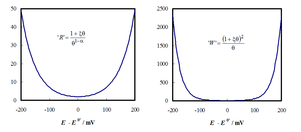
Figure 8.12. Potential dependency of charge transfer resistance (left) and Warburg element (right) without their constants. \( \xi \) = 1 and n = 1; \( \theta \) = exp[(nF)/(RT)(E - E0’)].
The value of the Warburg element becomes two orders of magnitude greater than that of the charge transfer resistance when the system is polarized, i.e. mass transfer to the electrode will be a limiting factor as shown in Figure 8.12. This is another reason why impedance measurements should not be conducted with high overpotential values.