CHEM-E4175 - Fundamental Electrochemistry, 09.01.2019-18.02.2019
This course space end date is set to 18.02.2019 Search Courses: CHEM-E4175
Kirja
8. Impedance technique
8.7. Dispersion of time constants
One of the key concepts in the impedance analysis is the time constant. As we have seen earlier, a resistor and a capacitor are always paired, and when impedance is determined, the result includes terms with the product RC. The dimension of this product is actually a second, and thus the constant is defined as \( \tau \) = RC. The dimension of the quotient L/R is also a second, but such terms do not exist. We therefore usually say that the circuit in Figure 8.4 is characterized by one time constant, but the circuit in Figure 8.15 has two time constants. The number of the time constants is therefore equal to the number of semicircles in the impedance plot. In the combination of R and C in series, the semicircle is seen in the admittance plot. If the time constants are almost equal in magnitude, it can be difficult to distinguish between them.
In
practice, the semicircles observed are rarely perfect, but they seem to be
flattened in the imaginary direction. The phenomenon is taken into account by replacing C with a constant phase element (CPE), for which the admittance is
| \( Y=Y_0(j\omega)^\alpha \) |
(8.91) |
|---|
The range of the factor a, i.e. the frequency in Equation (8.88) is in
theory [-1,1], but in practice [0,1]. If \( \alpha \) =
0, CPE is a resistor and Y0 = 1/R. When \( \alpha \) = 0.5, CPE corresponds to the Warburg element,
and \( Y_0=\sqrt2/\sigma \) (see (8.22)). If \( \alpha \) = 1, CPE is a capacitor and Y0 = C. If \( \alpha \) = -1, CPE is an inductor, and Y0
= L-1. The name constant phase element derives from the fact that the angle
of the impedance vector is constant independent of frequency:
| \( j^\alpha=(e^{j \pi/2})^\alpha=e^{j \alpha \pi/2}=\cos(\alpha \pi/2)+j\sin(\alpha \pi/2) \) | (8.92) |
|---|
The flattened semicircle in the impedance plot is obtained when \( \alpha \) < 1. Simulated R-CPE circuits with three different values of a are shown in Figure 8.22. The figure illustrates that the smaller \( \alpha \), the more the semicircle is flattened.
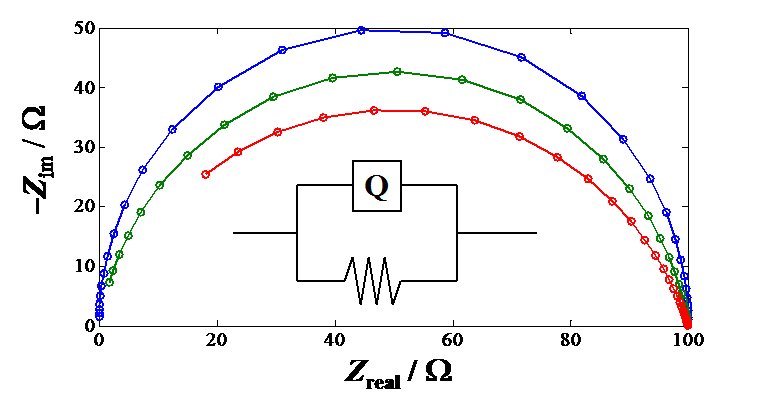
Figure 8.22. Impedance plots of a constant phase element and a resistor in parallel with values of \( \alpha \) = 1, 0.9 and 0.8; R = 100 \( \Omega \) and Y0 = 10-7 \( \Omega \)-1. The symbol Q describes the CPE in the fitting software.
In practice, the angle of 45 degrees, which corresponds to the Warburg element, is not reached either, but it remains smaller. In this case, the Warburg element is replaced by CPE, where \( \alpha \) < 0.5. Even though it is mathematically possible to take into account the descent of the semicircle and the inclination of the Warburg line using CPE, for every CPE there will be one parameter more in the mathematical treatment. Because of this, it is harder for the iteration to converge, and thus the model may produce erroneous results.
Naturally,
the next question we want to ask is about the physical source or interpretation of
CPE. The answer lies in the heterogeneity of the electrode surface. First, the
surface is far from being completely smooth. Instead, it is rough at least at
a molecular level, and usually also at a micrometer level. Second, the
electrode surface is not chemically completely heterogeneous either, but it may
contain oxidized passive domains or very active areas, for example at the boundaries
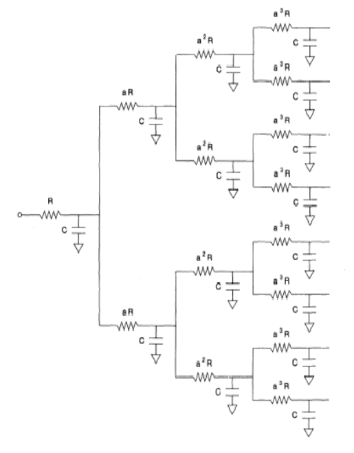
of crystal surfaces. Because of this, the reaction rate constant and the
corresponding charge transfer resistance do not have one single value, but a
distribution of values at different points on the surfaces. As a result, the
circuit does not have one single time constant, but rather a distribution of time
constants. The equivalent circuit of the case is illustrated in Figure 8.23.
The
diffusion element is affected by the surface roughness in a different manner. If
the surface of the electrode were completely smooth, the concentration at a
given distance from the surface would be constant. But if the surface is rough,
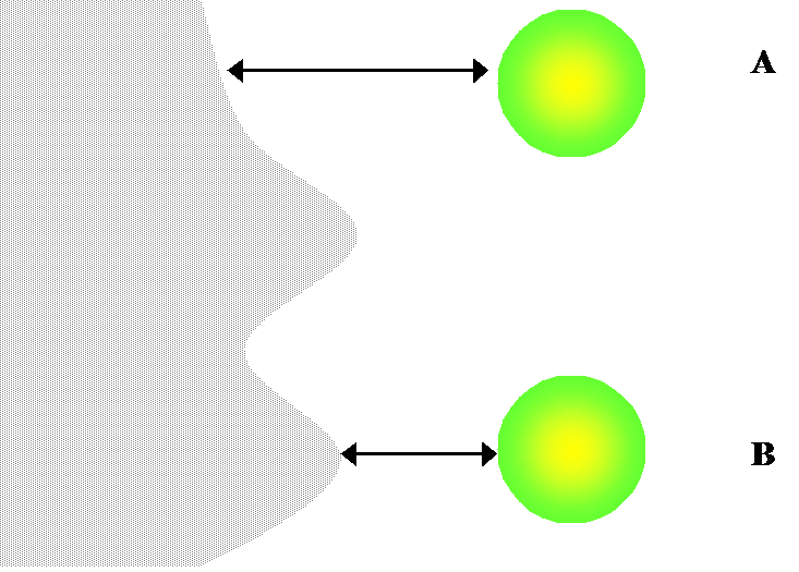
there will be equi-concentration planes near the surface of the electrode. Consider Figure 8.24. At a molecular level, diffusion can be seen as Brownian
motion. The probability of our test particle hitting the surface of the
electrode during a time step Dt is greater at point B than at point A.
On the other hand, the average time for the particle to reach the surface is
shorter at point B than at point A. The total current
observed in experiments therefore provides information on the surface roughness with
respect to the average diffusion distance \( l \sim\sqrt{D\Delta t} \). This is seen
in the potential step experiments (Chapter 7) as the current does not decrease \( \sim t^{-1/2} \) but is a bit
more gradual, and also the inclination of the Warburg line is lower.
It is evident that the more heterogeneous the surface,
the lower the value of \( \alpha \). However, the
heterogeneity of the surface can be evaluated in a more analytical manner.
It has been suggested [1]
that the frequency exponential of the CPE \( \alpha \) and the fractal dimension DF
are related as
Looking at Equation (8.93) it is obvious that because the dimension of the euclidic surface is 2, \( \alpha \) is equal to 1. The fractal dimensions of physical surfaces are in the range 2.1-2.3, which means that the range of a is 0.77-0.91, which is exactly what we observe in measurements. At the frequency range of diffusion, the Warburg element is replaced by the CPE with \( \alpha \) < 0.5. In this case, the relation has been suggested to be [2]
From Equation (8.94) it is seen that if \( \alpha \) < 0.5, DF < 2. Because of this, it is a bit confusing that the same surface gives DF > 2 at the frequency range of CPE, and DF < 2 at the frequencies of diffusion. However, these different processes are observed at different ranges of frequencies. It is necessary to keep in mind that the fractal nature of the surface is not solely its roughness, but the fractals are required to be similar, which means that the shape of the surface must be replicated at all magnifications. In practice, this cannot be the case, but the characteristics of the surface must be repeated at least in four different orders of magnitude in order for the surface to be fractal. |
|---|
[1] T. Pajkossy, L. Nyikos, J. Electrochem. Soc. 133 (1986) 2061.
[2] A.P. Borosy, L. Nyikos, T, Pajkossy, Electrochim. Acta 36 (1990) 163.