CHEM-E4175 - Fundamental Electrochemistry, 09.01.2019-18.02.2019
This course space end date is set to 18.02.2019 Search Courses: CHEM-E4175
Kirja
1. Electrochemical system
1.3. Properties of electrodes
1.3.1 Electron structure of solid materials
Electrodes are typically solid, metallic materials. In order to understand reactions taking place on them, it is useful to examine the structure of solid metals. A simple approach is to consider the structure as an ensemble of tightly packed lattices of atomic nuclei and electrons that are partly moving freely within the lattice. Let us concentrate on the cloud of these free electrons and study its emergence with an example. Lithium is the lightest alkali metal, its electron configuration is 1s22s1. It has one electron more than a noble gas (e.g. He). Two lithium atoms form a molecule Li2. The molecular orbital theory tells that from the two atomic 2s orbitals of lithium, two molecular orbitals are formed in a Li2 molecule: a binding orbital \( \sigma \)2s that resides between the Li nuclei, and an anti-bonding orbital \( \sigma \)*2 s on the opposite sides of the nuclei. According to the Aufbau principle, the 2s electrons of the lithium atoms that participate in the bond formation are filling the binding molecular orbital; the four 1s electrons stay on their atomic orbitals. Bringing more Li atoms into the system means more molecular orbitals are formed, including anti-bonding orbitals. Upon this process, the energy levels of the bonding orbitals get closer to each other, ultimately forming a continuous energy band when the number of atoms becomes high (molecule LiN), see Figure 1.2. Binding electrons, one electron for each Li atom, occupy only half of this band known as the valence band.
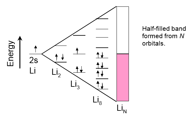
In terms of energy, below the valence band there is a band of 1s electrons that is fully occupied (not shown in Figure 1.2). Between this band and the valence band, there is an energy gap that is so wide that no 1s electron can rise to the valence band. Above the valence band there is a conduction band that is unoccupied at ground state. (Figures 1.2 and 1.3). In the case of lithium, it is formed from the molecular orbitals that are left unoccupied. Their energy is higher than that of the occupied orbitals by such small an amount that thermal energy (kBT) is capable of raising electrons to them, making lithium electronically conducting. Metals, in general, are good electronic conductors because their valence electrons are delocalized within the entire lattice.
Considering alkaline earth metals such as
magnesium in the similar manner, the situation changes somewhat. Molecular
orbitals formed from atomic 3s orbitals would be fully occupied by the 3s
electrons of Mg. So why are alkaline earth metals also good electronic conductors? Let us continue with the example
of Mg. Molecular orbitals are also formed from the atomic orbitals that are unoccupied at ground state (3p orbitals). Again, when the number of atoms is
high, the energy levels of these unoccupied molecular orbitals form a continuous
band. In magnesium, this band partly overlaps with the valence band, making the
exchange of electrons between the valence and conduction band feasible, see Figure
1.3.
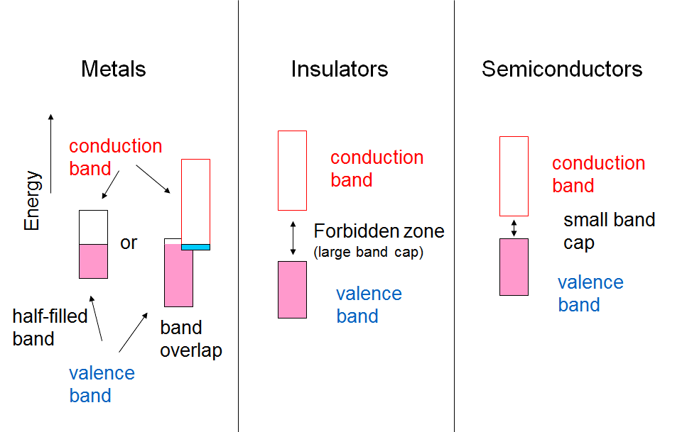
Electrical conductivity can be reduced to the issue of the band gap between the valence and conduction bands, as shown in Figure 1.3. If the band gap is of the order of 5 eV or higher, the material is an insulator because thermal energy (kBT = 0.025 eV at 300 K) is not capable of raising an electron from the valence band to the conduction band. If the band gap is of the order of 1-2 eV, some electrons can be raised to the conduction band, and the material is a semi-conductor. The conductivity of semi-conductors increases with temperature, in other words thermal energy, while the conductivity of metals decreases because the thermal motion of the metal nuclei interferes the free transfer of electrons. This is used as the definition of a metal.
1.3.2 Fermi levels and work function in solids
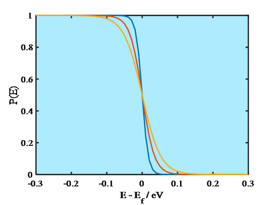
Electrons are fermions obeying the Pauli exclusion principle that two electrons cannot have the same quantum state in a system. As the consequence, electrons do not occupy the energy levels according to the Boltzmann but the Fermi-Dirac distribution. The probability P of finding an electron on an energy level E is
| \( \displaystyle P(E)=\frac{1}{1+e^{(E-E_f)/kT}} \) | (1.8) |
|---|
where Ef is the Fermi energy. At absolute zero (0 K) the energy levels are occupied according to the Aufbau principle, starting from the lowest energy level. The energy of the highest occupied molecular orbital, HOMO, is known as the Fermi energy that is also equal to the electrochemical potential of an electron. As Equation (1.8) manifests, at 0 K the probability of finding an electron on an energy level E < Ef is unity and on a level E > Ef zero. Since the electrochemical potential of an electron in a metal does not change significantly as a function of temperature, it has been common to call the energy where the step function occurs the Fermi level. At higher temperatures, however, Fermi-Dirac distribution is no longer a step function but changes smoothly, as shown in Figure 1.4. Yet, the distribution takes values different from unity or zero only around the energy where P(E) = 0.5, which is the definition of the Fermi level. The Fermi level is sometimes defined as the lowest energy of the conduction band of a solid which makes it possible to give numerical values to the Fermi level with respect to a reference point.
In solid state physics, metals are often sorted according to their work function, \( \Phi \), which is the work (energy) required to remove an electron from an uncharged metal, that is, from its Fermi level. The work function can be measured via, for example, the photoelectric effect. The work function is in practice a temperature-independent quantity, but it is important to note that it does depend on the lattice structure of a material. Work functions of metals vary from 2.3 eV of potassium to 5.3 eV of gold.
1.3.3 Potential and voltage
Potential is one of the most versatile and salient quantities in electrochemistry. Voltage is often used as a synonym for potential, but voltage is a measurable quantity while only potential differences can (possibly) be measured. Voltage can thus be defined as the potential difference between two points that can be a sum of several contributions. The free energy of the net electrochemical reaction is converted to the cell voltage according to Equation (1.6) which is the sum of the contributions of the anode and cathode reactions. Free energy is the driving force of a reaction and a measure of its tendency to take place, and we know from thermodynamics that spontaneous reactions have negative Gibbs free energies. Therefore, from Equation (1.6), positive cell voltages mean spontaneous reactions that produce energy, for example in a battery.
Although thermodynamics is not capable of resolving the free energy of individual electrode reactions, but an assumption is made to fix the potential scale (Chapter 4), we can elaborate the potential of a solid electrode a little bit further. The potential of a solid electrode – be it metal or semiconductor – can be considered a measure of the Fermi level of electrons in the electrode. From electrostatics we know that an extra electric charge creates potential. If an electrode carries a net negative charge its potential is negative with respect to an uncharged electrode or to an electroneutral solution. A positive charge obviously means positive potential. With electrochemical instrumentation, we can control the electrode potential externally which means controlling the Fermi levels or, alternatively, the charge of an electrode.
Let us consider further potential related quantities encountered in electrochemistry. The inner phase of any material is electroneutral. If an object carries an electric charge it is spread over its surface. The potential measured on the surface of an object or in its immediate proximity, with respect to vacuum, is the outer potential, \( \ \psi \). This is the work required to bring an elementary charge from an infinite distance in a vacuum to the surface of a phase (see Figure 1.5). The outer potential can be measured using a Kelvin probe. It follows from the previous paragraph that a negatively charged object has a negative outer potential and a positively charged one a positive outer potential. The potential difference between two charged objects is also known as the Volta potential difference.
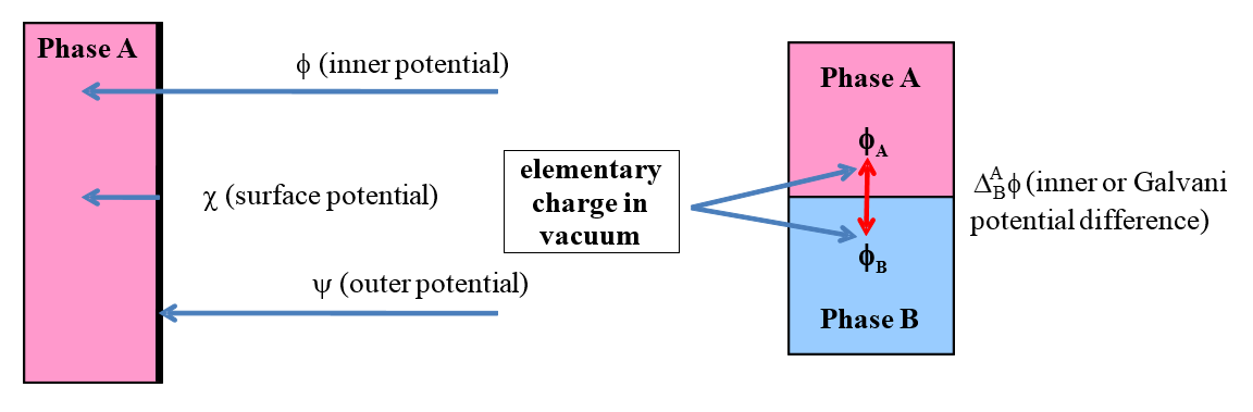
Figure 1.5. Left: Definitions of the inner or Galvani potential (\( \phi \)), surface potential (\( \ \chi \)) and outer potential (\( \psi \)). Right: Galvani potential difference between two phases.
\( \chi \) is the surface potential, the work required to bring an elementary charge from the surface of an object into its interior. The surface potential cannot be measured. The origin of the surface potential is the difference in the molecular (or atomic) interactions on the surface and in the interior of a material. In solids and liquids, molecules (atoms) residing on the surface experience asymmetric attraction towards the interior that gives them higher energy than that of the bulk of the material. Inserting a charged electrode into a polar solvent, the solvent molecules are oriented in a particular manner, creating surface dipoles. Now surface potential is created across the layer of these dipoles. The inner or Galvani potential, \( \phi \), is the total work required to bring an elementary charge from a vacuum to the inside of a phase. Based on what is stated above (and Figure 1.5), the Galvani potential can be expressed as the sum of the outer and surface potentials:
| \( \phi=\psi+\chi \) | (1.9) |
|---|
Galvani potential cannot be measured. On the right of Figure 1.5, the Galvani potential difference is defined. That can be measured under certain experimental arrangements (Chapter 4). Because the interiors of the both phases are electroneutral, Galvani potentials are constant within the materials and the Galvani potential difference is always formed at the interface between the phases.
1.3.4 Electron transfer on an electrode
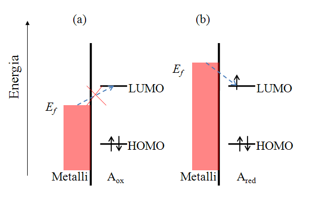
Let us consider the reduction reaction (1.2a) in a qualitative manner. Species A has an electronic structure based on the molecular orbital theory, as depicted in Figure 1.6. In order to reduce A, an electron must be transferred to its lowest unoccupied molecular orbital (LUMO). In Figure 1.6a, the Fermi level of the electrode is not sufficiently high to inject an electron to A, but as the electrode potential is changed so that the Fermi level is set higher than that of the LUMO of A (Figure 1.6b), and electron transfer becomes feasible. It is necessary to emphasize that an electron in the solution, or merely in the solute dissolved in the solvent, has no unambiguously defined energy. It is commonly assumed that its energy demonstrates Gaussian distribution and depends on the solvent-solute interactions. The Fermi level of an electron in the solution is defined as its electrochemical potential (see Chapter 6).
The rates of electron transfer can vary in the range of several orders of magnitude. This property can be quantified as the polarizability of an electrode. Polarizability is simply a measure of the dependence of the electron transfer rate on the electrode potential. An ideally non-polarizable electrode does not change its potential when current is flowing through it, while the potential of an ideally polarizable electrode can be varied without current flowing, see Figure 1.7.
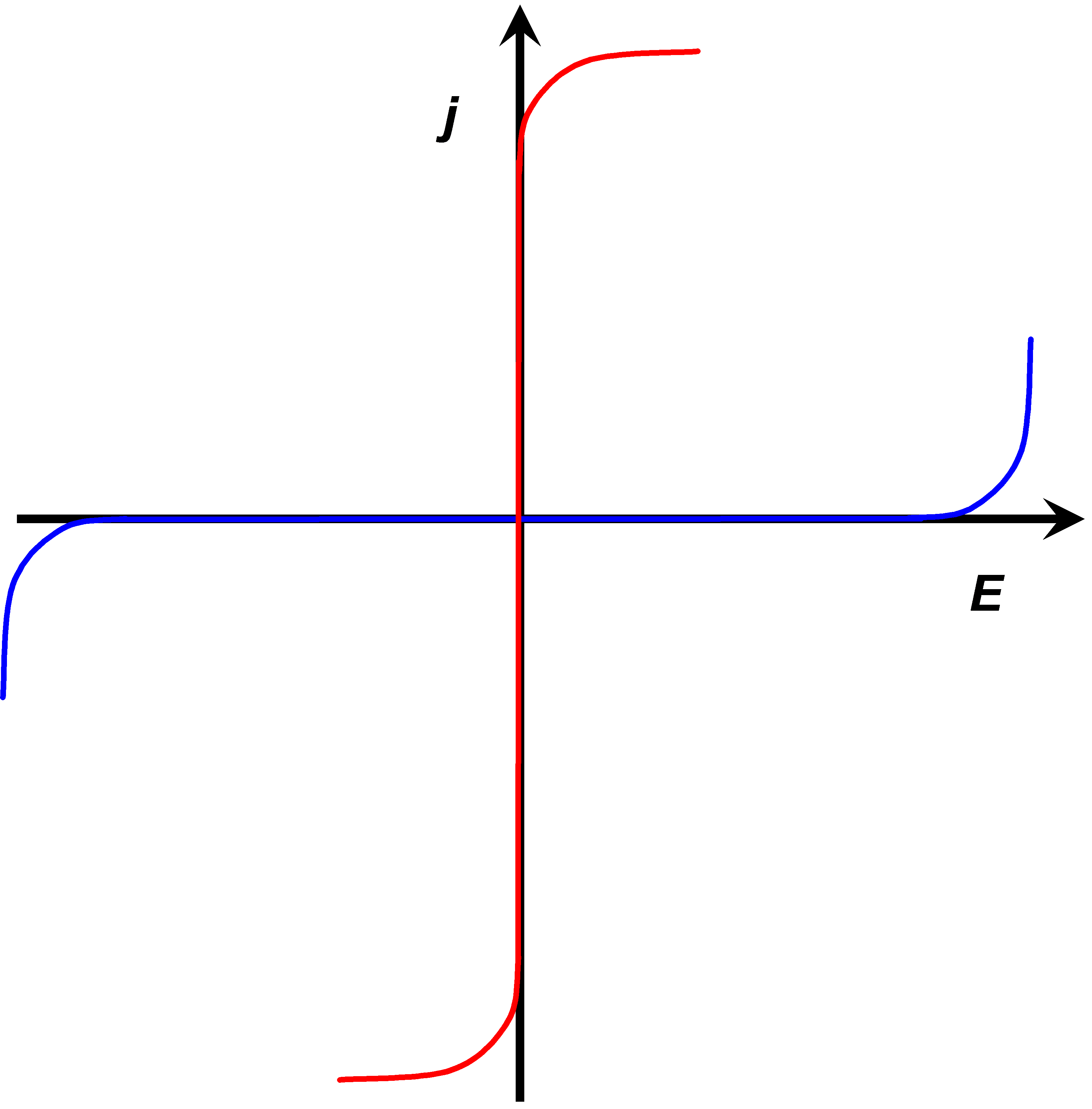
The rate of electron transfer in an ideally non-polarizable electrode is infinitely high, while the rate in an ideally polarizable electrode is zero. Ideal electrodes do not naturally exist but a Ag/AgCl electrode is non-polarizable to a significant extent. Its exchange current density (see paragraph 6.2.2) can be as high as 10 A cm–2. Perhaps the best polarizable electrode is the mercury drop. Its potential can be varied in the range of ca. 2.5 V without electrode reactions. The range of this potential window is determined by water splitting that is kinetically hindered on mercury. The electrode surface can also be modified in order to make it polarizable. Grafting an inert chemical group onto the surface, such as the diazonium moiety on graphite, the potential window can be extended to almost 4 V.
You can now test your conceptual knowledge by taking Quiz Chapter 1.